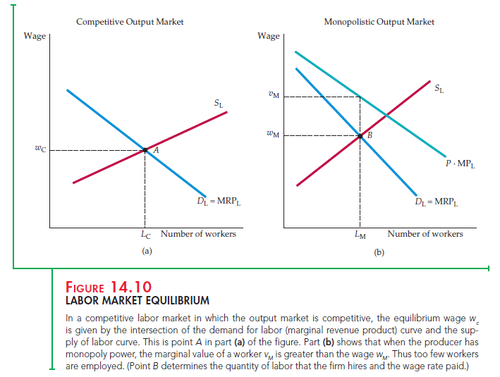
A competitive factor market is in equilibrium when the price of the input equates the quantity demanded to the quantity supplied. Figure 14.10 (a) shows such an equilibrium for a labor market. At point A, the equilibrium wage rate is wC and the equilibrium quantity supplied is L. Because they are well informed, all workers receive the identical wage and generate the identical marginal revenue product of labor wherever they are employed. If any worker had a wage lower than her marginal product, a firm would find it profitable to offer that worker a higher wage.
If the output market is also perfectly competitive, the demand curve for an input measures the benefit that consumers of the product place on the additional use of the input in the production process. The wage rate also reflects the cost to the firm and to society of using an additional unit of the input. Thus, at A in Figure 14.10 (a), the marginal benefit of an hour of labor (its marginal revenue product MRPl) is equal to its marginal cost (the wage rate w).
When output and input markets are both perfectly competitive, resources are used efficiently because the difference between total benefits and total costs is maximized. Efficiency requires that the additional revenue generated by employing an additional unit of labor (the marginal revenue product of labor, MRPl) equal the benefit to consumers of the additional output, which is given by the price of the product times the marginal product of labor, (P)(MPl).
When the output market is not perfectly competitive, the condition MRPl = (P)(MPl) no longer holds. Note in Figure 14.10 (b) that the curve representing the product price multiplied by the marginal product of labor [(P)(MPl)] lies above the marginal revenue product curve [(MR)(MPl)]. Point B is the equilibrium wage wM and the equilibrium labor supply LM. But because the price of the product is a measure of the value to consumers of each additional unit of output that they buy, (P)(MPl) is the value that consumers place on additional units of labor. Therefore, when LM laborers are employed, the marginal cost to the firm wM is less than the marginal benefit to consumers vM. Although the firm is maximizing its profit, its output is below the efficient level and it uses less than the efficient level of the input. Economic efficiency would be increased if more laborers were hired and, consequently, more output produced. (The gains to consumers would outweigh the firm’s lost profit.)
1. Economic Rent
The concept of economic rent helps explain how factor markets work. When discussing output markets in the long run in Chapter 8, we defined economic rent as the payments received by a firm over and above the minimum cost of producing its output. For a factor market, economic rent is the difference between the payments made to a factor of production and the minimum amount that must be spent to obtain the use of that factor. Figure 14.11 illustrates the concept of economic rent as applied to a competitive labor market. The equilibrium price of labor is w*, and the quantity of labor supplied is L*. The supply of labor curve is the upward-sloping curve, and the demand for labor is the downward-sloping marginal revenue product curve. Because the supply curve tells us how much labor will be supplied at each wage rate, the minimum expenditure needed to employ L* units of labor is given by the tan-shaded area AL*0B, below the supply curve to the left of the equilibrium labor supply L*.
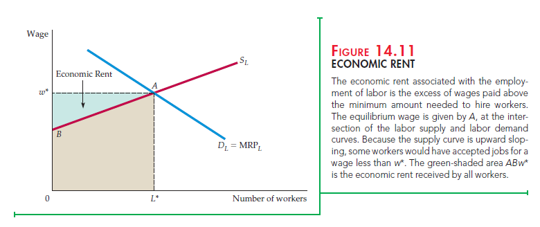
In perfectly competitive markets, all workers are paid the wage w*. This wage is required to get the last “marginal” worker to supply his or her labor, but all other workers earn rents because their wage is greater than the wage that would be needed to get them to work. Because total wage payments are equal to the rectangle 0w*AL*, the economic rent earned by labor is given by the area ABw*.
Note that if the supply curve were perfectly elastic, economic rent would be zero. There are rents only when supply is somewhat inelastic. And when supply is perfectly inelastic, all payments to a factor of production are economic rents because the factor will be supplied no matter what price is paid.
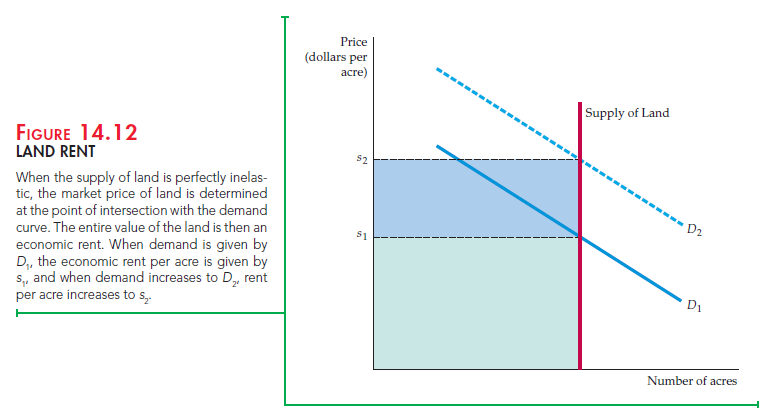
As Figure 14.12 shows, one example of an inelastically supplied factor is land. The supply curve is perfectly inelastic because land for housing (or for agriculture) is fixed, at least in the short run. With land inelastically supplied, its price is determined entirely by demand. The demand for land is given by D1, and its price per unit is sr Total land rent is given by the green-shaded rectangle. But when the demand for land increases to D2, the rental value per unit of land increases to s2; in this case, total land rent includes the blue-shaded area as well. Thus, an increase in the demand for land (a shift to the right in the demand curve) leads both to a higher price per acre and to a higher economic rent.
Source: Pindyck Robert, Rubinfeld Daniel (2012), Microeconomics, Pearson, 8th edition.
Just what I was looking for, regards for putting up.