Having described the conditions required to achieve an efficient allocation in the exchange of two goods, we now consider the efficient use of inputs in the production process. We assume that there are fixed total supplies of two inputs, labor and capital, which are needed to produce the same two products, food and clothing. Instead of only two people, however, we now assume that many consumers own the inputs to production (including labor) and earn income by selling them. This income, in turn, is allocated between the two goods.
This framework links the various supply and demand elements of the economy. People supply inputs to production and then use the income they earn to demand and consume goods and services. When the price of one input increases, the individuals who supply a lot of that input earn more income and consume more of one of the two goods. In turn, this increases the demand for the inputs needed to produce the good and has a feedback effect on the price of those inputs. Only a general equilibrium analysis can find the prices that equate supply and demand in every market.
1. Input Efficiency
To see how inputs can be combined efficiently, we must find the various combinations of inputs that can be used to produce each of the two outputs. A particular allocation of inputs into the production process is technically efficient if the output of one good cannot be increased without decreasing the output of another good. Because technical efficiency requires the appropriate combination of inputs, we will also call it input efficiency. Efficiency in production is not a new concept; in Chapter 6 we saw that a production function represents the maximum output that can be achieved with a given set of inputs. Here we extend the concept to the production of two goods rather than one.
If input markets are competitive, a point of efficient production will be achieved. Let’s see why. If the labor and capital markets are perfectly competitive, then the wage rate w will be the same in all industries. Likewise, the rental rate of capital r will be the same whether capital is used in the food or clothing industry. We know from Chapter 7 that if producers of food and clothing minimize production costs, they will use combinations of labor and capital so that the ratio of the marginal products of the two inputs is equal to the ratio of the input prices:
![]()
But we also showed that the ratio of the marginal products of the two inputs is equal to the marginal rate of technical substitution of labor for capital MRTStr As a result,
Because the MRTS is the slope of the firm’s isoquant, a competitive equilibrium can occur in the input market only if each producer uses labor and capital so that the slopes of the isoquants are equal to one another and to the ratio of the prices of the two inputs. As a result, the competitive equilibrium is efficient in production.
2. The Production Possibilities Frontier
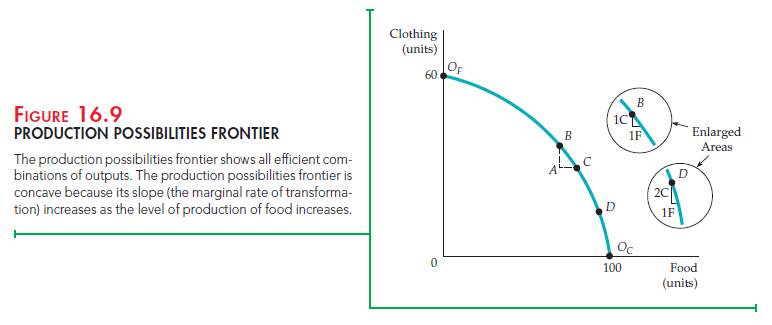
The production possibilities frontier shows the various combinations of food and clothing that can be produced with fixed inputs of labor and capital, holding technology constant. The frontier in Figure 16.9 is derived from the production contract curve. Each point on both the contract curve and the production possibilities frontier describes an efficiently produced level of both food and clothing.
Point OF represents one extreme, in which only clothing is produced, and OC represents the other extreme, in which only food is produced. Points B, C, and D correspond to points at which both food and clothing are efficiently produced.
Point A, representing an inefficient allocation, lies inside the production possibilities frontier. All points within the triangle ABC involve the complete utilization of labor and capital in the production process. However, a distortion in the labor market, perhaps due to a rent-maximizing union, has caused the economy as a whole to be productively inefficient.
Where we end up on the production possibilities frontier depends on consumer demand for the two goods. For example, suppose consumers tend to prefer food rather than clothing. A possible competitive equilibrium occurs at D in Figure 16.8. On the other hand, if consumers prefer clothing to food, the competitive equilibrium will occur on a point on the production possibilities frontier closer to OF.
Why is the production possibilities frontier downward sloping? In order to produce more food efficiently, one must switch inputs from the production of clothing, which in turn lowers the clothing production level. Because all points lying within the frontier are inefficient, they are off the production contract curve.
MARGINAL RATE OF TRANSFORMATION The production possibilities frontier is concave (bowed out)—i.e., its slope increases in magnitude as more food is produced. To describe this, we define the marginal rate of transformation of food for clothing (MRT) as the magnitude of the slope of the frontier at each point. The MRT measures how much clothing must be given up to produce one additional unit of food. For example, the enlarged areas of Figure 16.9 show that at B on the frontier, the MRT is 1 because 1 unit of clothing must be given up to obtain 1 additional unit of food. At D, however, the MRT is 2 because 2 units of clothing must be given up to obtain 1 more unit of food.
Note that as we increase the production of food by moving along the production possibilities frontier, the MRT increases.[1] This increase occurs because the productivity of labor and capital differs depending on whether the inputs are used to produce more food or clothing. Suppose we begin at OF, where only clothing is produced. Now we remove some labor and capital from clothing production, where their marginal products are relatively low, and put them into food production, where their marginal products are high. Under these circumstances, to obtain the first unit of food, very little clothing production is lost. (The MRT is much less than 1.) But as we move along the frontier and produce less clothing, the productivities of labor and capital in clothing production rise and the productivities of labor and capital in food production fall. At B, the productivities are equal and the MRT is 1. Continuing along the frontier, we note that because the input productivities in clothing rise more and the productivities in food decrease, the MRT becomes greater than 1.
We can also describe the shape of the production possibilities frontier in terms of the costs of production. At OF, where very little clothing output is lost to produce additional food, the marginal cost of producing food is very low: A lot of output is produced with very little input. Conversely, the marginal cost of producing clothing is very high: It takes a lot of both inputs to produce another unit of clothing. Thus, when the MRT is low, so is the ratio of the marginal cost of producing food MCF to the marginal cost of producing clothing MCC. In fact, the slope of the production possibilities frontier measures the marginal cost of producing one good relative to the marginal cost of producing the other. The curvature of the production possibilities frontier follows directly from the fact that the marginal cost of producing food relative to the marginal cost of producing clothing is increasing. At every point along the frontier, the following condition holds:
MRT = MCf/MCc (16.3)
At B, for example, the MRT is equal to 1. Here, when inputs are switched from clothing to food production, 1 unit of output is lost and 1 is gained. If the input cost of producing 1 unit of either good is $100, the ratio of the marginal costs would be $100/$100, or 1. Equation (16.3) also holds at D (and at every other point on the frontier). Suppose the inputs needed to produce 1 unit of food cost $160. The marginal cost of food would be $160, but the marginal cost of clothing would be only $80 ($160/2 units of clothing). As a result, the ratio of the marginal costs, 2, is equal to the MRT.
3. Output Efficiency
For an economy to be efficient, goods must not only be produced at minimum cost; goods must also be produced in combinations that match people’s willingness to pay for them. To understand this principle, recall from Chapter 3 that the marginal rate of substitution of clothing for food (MRS) measures the consumer’s willingness to pay for an additional unit of food by consuming less clothing. The marginal rate of transformation measures the cost of an additional unit of food in terms of producing less clothing. An economy produces output efficiently only if, for each consumer,
MRS = MRT (16.4)
To see why this condition is necessary for efficiency, suppose the MRT equals 1, while the MRS equals 2. In that case, consumers are willing to give up 2 units of clothing to get 1 unit of food, but the cost of getting the additional food is only 1 unit of lost clothing. Clearly, too little food is being produced. To achieve efficiency, food production must be increased until the MRS falls and the MRT increases and the two are equal. The outcome is output efficient only when MRS = MRT for all pairs of goods.
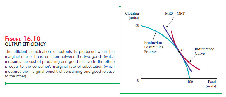
Figure 16.10 shows this important output efficiency condition graphically. Here, we have superimposed one consumer’s indifference curve on the production possibilities frontier from Figure 16.9. Note that C is the only point on the production possibilities frontier that maximizes the consumer’s satisfaction. Although all points on the production frontier are technically efficient, not all involve the most efficient production of goods from the consumer’s perspective. At the point of tangency of the indifference curve and the production frontier, the MRS (the slope of the indifference curve) and the MRT (the slope of the production frontier) are equal.
If you were a planner in charge of managing an economy, you would face a difficult problem. To achieve output efficiency, you must equate the marginal rate of transformation with the consumer’s marginal rate of substitution. But if different consumers have different preferences for food and clothing, how can you decide what levels of food and clothing to produce and what amount of each to give to every consumer, so that all consumers have the same MRS? The informational and logistical costs are enormous. That is one reason why centrally planned economies, like that of the former Soviet Union, performed so poorly. Fortunately, a well-functioning competitive market system can achieve the same efficient outcome as an ideal managed economy.
4. Efficiency in Output Markets
When output markets are perfectly competitive, all consumers allocate their budgets so that their marginal rates of substitution between two goods are equal to the price ratio. For our two goods, food and clothing,
MRS = PF/PC
At the same time, each profit-maximizing firm will produce its output up to the point at which price is equal to marginal cost. Again, for our two goods,
Pf = MCf and Pc=MCc
Because the marginal rate of transformation is equal to the ratio of the marginal costs of production, it follows that
MRT = MCf/MCc = PF/PC = MRS (16.5)
When output and input markets are competitive, production will be output efficient in that the MRT is equal to the MRS. This condition is just another version of the marginal benefit-marginal cost rule discussed in Chapter 4. There we saw that consumers buy additional units of a good up to the point at which the marginal benefit of consumption is equal to the marginal cost. Here we see that the production of food and clothing is chosen so that the marginal benefit of consuming another unit of food is equal to the marginal cost of producing another unit of food; the same is true for the consumption and production of clothing.
Figure 16.11 shows that efficient competitive output markets are achieved when production and consumption choices are separated. Suppose the market generates a price ratio of P’F/P’c. If producers are using inputs efficiently, they will produce food and clothing at A, where the price ratio is equal to the MRT, the slope of the production possibilities frontier. When faced with this budget constraint, however, consumers would like to consume at B, where they maximize their satisfaction at the higher indifference curve U2. However, at the price ratio Pf/Pc, producers will not produce the combination of food and clothing at B. Because the producer wants to produce F1 units of food, while consumers want to buy F2, there will be an excess demand for food. Correspondingly, because consumers wish to buy C2 units of clothing while producers wish to sell Cv there will be an excess supply of clothing. Prices in the market will then adjust: The price of food will rise and that of clothing will fall. As price ratio Pf/Pc increases, the price line will move along the production frontier.
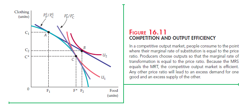
An equilibrium results when the price ratio is Pf/Pc at C. In equilibrium, there is no way to make a consumer better off without making another consumer worse off. Hence, this equilibrium is Pareto efficient. Moreover, producers want to sell F units of food and C* units of clothing; consumers want to buy the same amounts. At this equilibrium, the MRT and the MRS are equal again; therefore, the competitive equilibrium is output efficient.
Source: Pindyck Robert, Rubinfeld Daniel (2012), Microeconomics, Pearson, 8th edition.
Very interesting subject, thankyou for posting. “Nothing is more wretched than the mind of a man conscious of guilt.” by Titus Maccius Plautus.