So far, we have focused only on the first element of consumer theory—consumer preferences. We have seen how indifference curves (or, alternatively, utility func- tions) can be used to describe how consumers value various baskets of goods. Now we turn to the second element of consumer theory: the budget constraints that consumers face as a result of their limited incomes.
1. The Budget Line
To see how a budget constraint limits a consumer’s choices, let’s consider a situation in which a woman has a fixed amount of income, I, that can be spent on food and clothing. Let F be the amount of food purchased and C be the amount of clothing. We will denote the prices of the two goods PF and PC. In that case, PfF (i.e., price of food times the quantity) is the amount of money spent on food and PCC the amount of money spent on clothing.
The budget line indicates all combinations of F and C for which the total amount of money spent is equal to income. Because we are considering only two goods (and
t mncome ignoring the possibility of saving), our hypothetical consumer will spend her
entire income on food and clothing. As a result, the combinations of food and clothing that she can buy will all lie on this line:
PfF + PCC = I
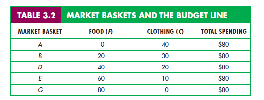
Suppose, for example, that our consumer has a weekly income of $80, the price of food is $1 per unit, and the price of clothing is $2 per unit. Table 3.2 shows various combinations of food and clothing that she can purchase each week with her $80. If her entire budget were allocated to clothing, the most that she could buy would be 40 units (at a price of $2 per unit), as represented by market basket A. If she spent her entire budget on food, she could buy 80 units (at $1 per unit), as given by market basket G. Market baskets B, D, and E show three additional ways in which her $80 could be spent on food and clothing.
Figure 3.10 shows the budget line associated with the market baskets given in Table 3.2. Because giving up a unit of clothing saves $2 and buying a unit of food costs $1, the amount of clothing given up for food along the budget line must be the same everywhere. As a result, the budget line is a straight line from point A to point G. In this particular case, the budget line is given by the equation F + 2C = $80.
The intercept of the budget line is represented by basket A. As our consumer moves along the line from basket A to basket G, she spends less on clothing and more on food. It is easy to see that the extra clothing which must be given up to consume an additional unit of food is given by the ratio of the price of food to the price of clothing ($1/$2 = 1/2). Because clothing costs $2 per unit and food only $1 per unit, 1/2 unit of clothing must be given up to get 1 unit of food. In Figure 3.10, the slope of the line, AC/AF = -1/2, measures the relative cost of food and clothing.

Using equation (3.1), we can see how much of C must be given up to consume more of F. We divide both sides of the equation by PC and then solve for C:
C = (I/Pc) – (Pf/Pc)F (3.2)
Equation (3.2) is the equation for a straight line; it has a vertical intercept of I/PC and a slope of -(Pf/Pc).
The slope of the budget line, -(Pf/Pc), is the negative of the ratio of the prices of the two goods. The magnitude of the slope tells us the rate at which the two goods can be substituted for each other without changing the total amount of money spent. The vertical intercept (I/Pc) represents the maximum amount of C that can be purchased with income I. Finally, the horizontal intercept (I/Pf ) tells us how many units of F can be purchased if all income were spent on F.
2. The Effects of Changes in Income and Prices
We have seen that the budget line depends both on income and on the prices of the goods, PF and PC. But of course prices and income often change. Let’s see how such changes affect the budget line.
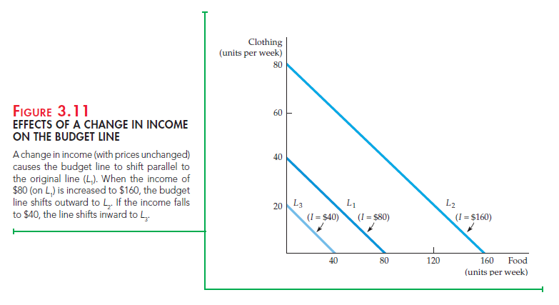
INCOME CHANGES What happens to the budget line when income changes? From the equation for the straight line (3.2), we can see that a change in income alters the vertical intercept of the budget line but does not change the slope (because the price of neither good changed). Figure 3.11 shows that if income is doubled (from $80 to $160), the budget line shifts outward, from budget line L1 to budget line L2. Note, however, that L2 remains parallel to L1. If she desires, our consumer can now double her purchases of both food and clothing. Likewise, if her income is cut in half (from $80 to $40), the budget line shifts inward, from L1 to L3.
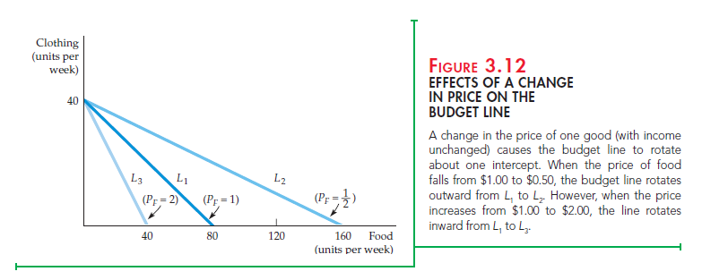
PRICE CHANGES What happens to the budget line if the price of one good changes but the price of the other does not? We can use the equation C = (I/PC) – (Pf/Pc)F to describe the effects of a change in the price of food on the budget line. Suppose the price of food falls by half, from $1 to $0.50. In that case, the vertical intercept of the budget line remains unchanged, although the slope changes from -Pf/Pc = —$1/$2 = —$1/2 to —$0.50/$2 = —$1/4. In Figure 3.12, we obtain the new budget line L2 by rotating the original budget line L1 outward, pivoting from the C-intercept. This rotation makes sense because a person who consumes only clothing and no food is unaffected by the price change. However, someone who consumes a large amount of food will experience an increase in his purchasing power. Because of the decline in the price of food, the maximum amount of food that can be purchased has doubled.
On the other hand, when the price of food doubles from $1 to $2, the budget line rotates inward to line L3 because the person’s purchasing power has diminished. Again, a person who consumed only clothing would be unaffected by the food price increase.
What happens if the prices of both food and clothing change, but in a way that leaves the ratio of the two prices unchanged? Because the slope of the budget line is equal to the ratio of the two prices, the slope will remain the same. The intercept of the budget line must shift so that the new line is parallel to the old one. For example, if the prices of both goods fall by half, then the slope of the budget line does not change. However, both intercepts double, and the budget line is shifted outward.
This exercise tells us something about the determinants of a consumer’s purchasing power—her ability to generate utility through the purchase of goods and services. Purchasing power is determined not only by income, but also by prices. For example, our consumer’s purchasing power can double either because her income doubles or because the prices of all the goods that she buys fall by half.
Finally, consider what happens if everything doubles—the prices of both food and clothing and the consumer’s income. (This can happen in an inflationary economy.) Because both prices have doubled, the ratio of the prices has not changed; neither, therefore, has the slope of the budget line. Because the price of clothing has doubled along with income, the maximum amount of clothing that can be purchased (represented by the vertical intercept of the budget line) is unchanged. The same is true for food. Therefore, inflationary conditions in which all prices and income levels rise proportionately will not affect the consumer’s budget line or purchasing power.
Source: Pindyck Robert, Rubinfeld Daniel (2012), Microeconomics, Pearson, 8th edition.
Good article. I am dealing with many of these issues as well..