Correlation and Regression with SPSS – Problem 8.3: Correlation Matrix for Several Variables

If you have more than two ordinal or normally distributed variables that you want to correlate, the program will produce a matrix showing the correlation of each selected variable with each of the others. You could print a matrix scatterplot to check the linear relationship for each pair of variables (see Fig. 8.1). We did such a scatterplot (not shown) and found that the assumption of linearity was not markedly violated for this problem.

• What are the associations among the four variables visualization, scholastic aptitude test— math, grades in h.s., and math achievement?

Now, compute Pearson correlations among all pairs of the following scale/normal variables: visualization, scholastic aptitude test—math, grades in h.s., and math achievement. Move all four into the Variables box (see Fig. 8.6). Follow the procedures for Problem 8.2 outlined previously, except:

• Do not check Spearman (under Correlation Coefficients) but do check Pearson.
• For Options, click Means and standard deviations, and Exclude cases listwise. The latter will only use participants who have no missing data on any of these four variables.

This will produce Output 8.3. To see if you are doing the work right, compare your syntax and output to Output 8.3.

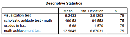
Output 8.3: Pearson Correlation Matrix

CORRELATIONS

/VARIABLES=visual satm grades mathach

/PRINT=TWOTAIL NOSIG

/STATISTICS DESCRIPTIVES /MISSING=LISTWISE .

Correlations

Interpretation of Output 8.3

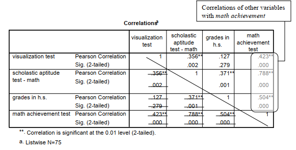
Notice that after the Descriptive Statistics table, there is a larger Correlations table that shows the Pearson Correlation coefficients and two-tailed significance (Sig.) levels. These numbers are, as in Output 8.2, each given twice so you have to be careful in reading the matrix. It is a good idea to look only at the numbers above (or below) the diagonal (the 1s). You can also benefit from drawing a similar line on your output, so that you will be sure to read only the upper or lower portion of the matrix. There are six different correlations in the table. In the last column, we have circled the correlation of each of the other variables with math achievement. In the second to last column, each of the other three variables is correlated with grades in h.s., but note that the .504 below the diagonal for grades in h.s. and math achievement is the same as the correlation of math achievement and grades in h.s. in the last column, so ignore it the second time.

The Pearson correlations on this table are interpreted similarly to the one in Output 8.2. However, because there are six correlations, the odds are increased that one could be statistically significant by chance. Thus, it would be prudent to require a smaller value of p. The Bonferroni correction is a conservative approach designed to keep the significance level at .05 for the whole study. Using Bonferroni, you would divide the usual significance level (.05) by the number of tests. In this case a p < .008 (.05/6) would be required for statistical significance. Another approach is simply to set alpha (the p value required for statistical significance) at a more conservative level, perhaps .01 instead of .05. Note that if we had checked Exclude cases pairwise in Fig. 8.6, the correlations would be the same, in this instance, because there were no missing data (N = 75) on any of the four variables. However, if some variables had missing data, the correlations would be at least somewhat different. Each correlation would be based on the cases that have no missing data on those two variables. One might use pairwise exclusion to include as many cases as possible in each correlation; however, the problem with this approach is that the correlations will include data from somewhat different individuals, making comparisons among correlations difficult. Multivariate statistics, such as multiple regression, use listwise exclusion, including only the subjects with no missing data.

If you checked One-Tailed Test of Significance in Fig. 8.6, the Pearson Correlation values would be the same as in Output 8.3, but the Sig. values would be half what they are here. For example, the Sig. for the correlation between visualization test and grades in h.s. would be .139 instead of .279. One-tailed tests are only used if you have a clear directional hypothesis (e.g., there will be a positive correlation between the variables). If one takes this approach, then all correlations in the direction opposite from that predicted must be ignored, even if they seem to be significant.

Example of How to Write About Problem 8.3

Results

Because each of the four achievement variables was normally distributed and the assumption of linearity was not markedly violated, Pearson correlations were computed to examine the intercorrelations of the variables. Table 8.1 shows that five of the six pairs of variables were significantly correlated. The strongest positive correlation, which would be considered a very large effect size according to Cohen (1988), was between the scholastic aptitude math test and math achievement test, r(73) = .79, p < .001. This means that students who had relatively high SAT math scores were very likely to have high math achievement test scores. Math achievement was also positively correlated with visualization test scores (r = .42) and grades in high school (r = .50); these are medium to large size effects or correlations according to Cohen (1988).

Table 8.1 Intercorrelations, Means, and Standard Deviations for Four Achievement Variables (N = 75)

Source: Morgan George A, Leech Nancy L., Gloeckner Gene W., Barrett Karen C.

(2012), IBM SPSS for Introductory Statistics: Use and Interpretation, Routledge; 5th edition; download Datasets and Materials.