Later in this book, we will explain how demand information is used as input into a firm’s economic decision-making process. General Motors, for example, must understand automobile demand to decide whether to offer rebates or below-market-rate loans for new cars. Knowledge about demand is also impor- tant for public policy decisions. Understanding the demand for oil, for instance, can help Congress decide whether to pass an oil import tax. You may wonder how it is that economists determine the shape of demand curves and how price and income elasticities of demand are actually calculated. In this starred section, we will briefly examine some methods for evaluating and forecasting demand. The section is starred not only because the material is more advanced, but also because it is not essential for much of the later analysis in the book. Nonetheless, this material is instructive and will help you appreciate the empirical founda- tion of the theory of consumer behavior. The basic statistical tools for estimating demand curves and demand elasticities are described in the appendix to this book, entitled “The Basics of Regression.”
1. The Statistical Approach to Demand Estimation
Firms often rely on market information based on actual studies of demand. Properly applied, the statistical approach to demand estimation can help researchers sort out the effects of variables, such as income and the prices of other products, on the quantity of a product demanded. Here we outline some of the conceptual issues involved in the statistical approach.
Table 4.6 shows the quantity of raspberries sold in a market each year. Information about the market demand for raspberries would be valuable to an organization representing growers because it would allow them to predict sales on the basis of their own estimates of price and other demand-determining vari- ables. Let’s suppose that, focusing on demand, researchers find that the quantity of raspberries produced is sensitive to weather conditions but not to the cur- rent market price (because farmers make their planting decisions based on last year ’s price).

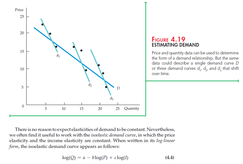
The price and quantity data from Table 4.6 are graphed in Figure 4.19. If we believe that price alone determines demand, it would be plausible to describe the demand for the product by drawing a straight line (or other appropriate curve), Q = a – bP, which “fit” the points as shown by demand curve D. (The “least- squares” method of curve-fitting is described in the appendix to the book.)
Does curve D (given by the equation Q = 28.2 – 1.00P) really represent the demand for the product? The answer is yes—but only if no important factors other than price affect demand. In Table 4.6, however, we have included data for one other variable: the average income of purchasers of the product. Note that income (I) has increased twice during the study, suggesting that the demand curve has shifted twice. Thus demand curves d1, d2, and d3 in Figure 4.19 give a more likely description of demand. This linear demand curve would be described algebraically as
Q = a – bP + cI (4.2)
The income term in the demand equation allows the demand curve to shift in a parallel fashion as income changes. The demand relationship, calculated using the least-squares method, is given by Q = 8.08 – .49P + .81I.
2. The Form of the Demand Relationship
Because the demand relationships discussed above are straight lines, the effect of a change in price on quantity demanded is constant. However, the price elasticity of demand varies with the price level. For the demand equation Q = a – bP, for example, the price elasticity EP is
Ep = (AQ/A P)(P/Q) = – b(P/Q) (4.3)
Thus elasticity increases in magnitude as the price increases (and the quantity demanded falls).
Consider, for example, the linear demand for raspberries, which was estimated to be Q = 8.08 – .49P + .81I. The elasticity of demand in 1999 (when Q = 16 and P = 10) is equal to -.49 (10/16) = -.31, whereas the elasticity in 2003 (when Q = 22 and P = 5) is substantially lower: -.11.
where log ( ) is the logarithmic function and a, b, and c are the constants in the demand equation. The appeal of the log-linear demand relationship is that the slope of the line -b is the price elasticity of demand and the constant c is the income elasticity.[1] Using the data in Table 4.5, for example, we obtained the regression line
log(Q) = -0.23 – 0.34 log(P) + 1.33 log(I)
This relationship tells us that the price elasticity of demand for raspberries is — 0.34 (that is, demand is inelastic), and that the income elasticity is 1.33.
We have seen that it can be useful to distinguish between goods that are complements and goods that are substitutes. Suppose that P2 represents the price of a second good—one which is believed to be related to the product we are studying. We can then write the demand function in the following form:
log(Q) = a – blog(P) + b2 log(P2) + c log(I)
When b2, the cross-price elasticity, is positive, the two goods are substitutes; when b2 is negative, the two goods are complements.
The specification and estimation of demand curves has been a rapidly growing endeavor, not only in marketing, but also in antitrust analyses. It is now commonplace to use estimated demand relationships to evaluate the likely effects of mergers.[1] What were once prohibitively costly analyses involving mainframe computers can now be carried out in a few seconds on a personal computer. Accordingly, governmental competition authorities and economic and marketing experts in the private sector make frequent use of supermarket scanner data as inputs for estimating demand relationships. Once the price elasticity of demand for a particular product is known, a firm can decide whether it is profitable to raise or lower price. Other things being equal, the lower in magnitude the elasticity, the more likely the profitability of a price increase.
Source: Pindyck Robert, Rubinfeld Daniel (2012), Microeconomics, Pearson, 8th edition.
Yay google is my world beater aided me to find this great internet site! .
I genuinely treasure your work, Great post.