Determining the Sample Size for a Hypothesis Test About a Population Mean

Assume that a hypothesis test is to be conducted about the value of a population mean. The level of significance specified by the user determines the probability of making a Type I error for the test. By controlling the sample size, the user can also control the probability of making a Type II error. Let us show how a sample size can be determined for the following lower tail test about a population mean.

The upper panel of Figure 9.10 is the sampling distribution of X when H₀ is true with μ = μ₀. For a lower tail test, the critical value of the test statistic is denoted -z_a. In the upper panel of the figure the vertical line, labeled c, is the corresponding value of X. Note that, if we reject H₀ when X ≤ c, the probability of a Type I error will be a. With z_a rep­resenting the z value corresponding to an area of a in the upper tail of the standard normal distribution, we compute c using the following formula:

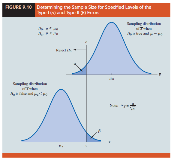
The lower panel of Figure 9.10 is the sampling distribution of X when the alternative hypothesis is true with μ = μ_a < μ₀. The shaded region shows b, the probability of a Type II error that the decision maker will be exposed to if the null hypothesis is accepted when X > c. With z_β representing the z value corresponding to an area of β in the upper tail of the standard normal distribution, we compute c using the following formula:

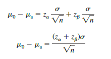
Now what we want to do is to select a value for c so that when we reject H₀ and accept H_a, the probability of a Type I error is equal to the chosen value of a and the probability of a Type II error is equal to the chosen value of β. Therefore, both equations (9.5) and (9.6) must provide the same value for c, and the following equation must be true.

To determine the required sample size, we first solve for the √n as follows.

and

Squaring both sides of the expression provides the following sample size formula for a one-tailed hypothesis test about a population mean.

Although the logic of equation (9.7) was developed for the hypothesis test shown in Figure 9.10, it holds for any one-tailed test about a population mean. In a two-tailed hypothesis test about a population mean, z_a/2 is used instead of z_a in equation (9.7).

Let us return to the lot-acceptance example from Sections 9.6 and 9.7. The design spe­cification for the shipment of batteries indicated a mean useful life of at least 120 hours for the batteries. Shipments were rejected if H₀: μ ≥ 120 was rejected. Let us assume that the quality control manager makes the following statements about the allowable probabilities for the Type I and Type II errors.

Type I error statement: If the mean life of the batteries in the shipment is μ = 120, I am willing to risk an a = .05 probability of rejecting the shipment.

Type II error statement: If the mean life of the batteries in the shipment is 5 hours under the specification (i.e., μ = 115), I am willing to risk a b = .10 probability of accepting the shipment.

These statements are based on the judgment of the manager. Someone else might specify different restrictions on the probabilities. However, statements about the allowable probab­ilities of both errors must be made before the sample size can be determined.

In the example, a = .05 and b = .10. Using the standard normal probability distribu­tion, we have z.₀₅ = 1.645 and z.₁₀ = 1.28. From the statements about the error probabilit­ies, we note that μ₀ = 120 and μ_a = 115. Finally, the population standard deviation was assumed known at σ = 12. By using equation (9.7), we find that the recommended sample size for the lot-acceptance example is

Rounding up, we recommend a sample size of 50.

Because both the Type I and Type II error probabilities have been controlled at allow­able levels with n = 50, the quality control manager is now justified in using the accept H₀ and reject H₀ statements for the hypothesis test. The accompanying inferences are made with allowable probabilities of making Type I and Type II errors.

We can make three observations about the relationship among a, b, and the sample size n.

1. Once two of the three values are known, the other can be computed.
2. For a given level of significance a, increasing the sample size will reduce b.
3. For a given sample size, decreasing a will increase b, whereas increasing a will decrease b.

The third observation should be kept in mind when the probability of a Type II error is not being controlled. It suggests that one should not choose unnecessarily small values for the level of significance a. For a given sample size, choosing a smaller level of signific­ance means more exposure to a Type II error. Inexperienced users of hypothesis testing often think that smaller values of a are always better. They are better if we are concerned only about making a Type I error. However, smaller values of a have the disadvantage of increasing the probability of making a Type II error.

Source:  Anderson David R., Sweeney Dennis J., Williams Thomas A. (2019), Statistics for Business & Economics, Cengage Learning; 14th edition.