Exponential Probability Distribution

The exponential probability distribution may be used for random variables such as the time between arrivals at a hospital emergency room, the time required to load a truck, the distance between major defects in a highway, and so on. The exponential probability density function follows.

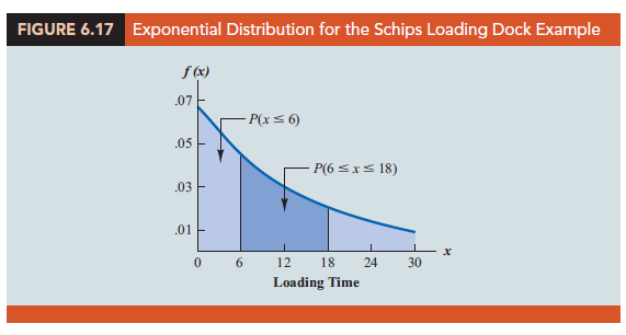
As an example of the exponential distribution, suppose that x represents the loading time for a truck at the Schips loading dock and follows such a distribution. If the mean, or average, loading time is 15 minutes (m = 15), the appropriate probability density function for x is

Figure 6.17 is the graph of this probability density function.

1. Computing Probabilities for the Exponential Distribution

As with any continuous probability distribution, the area under the curve corresponding to an interval provides the probability that the random variable assumes a value in that interval. In the Schips loading dock example, the probability that loading a truck will take 6 minutes or less, P(x < 6), is defined to be the area under the curve in Figure 6.17 from x = 0 to x = 6. Similarly, the probability that the loading time will be 18 minutes or less, P(x < 18), is the area under the curve from x = 0 to x = 18. Note also that the probability that the loading time will be between 6 minutes and 18 minutes, P(6 < x < 18), is given by the area under the curve from x = 6 to x = 18.

To compute exponential probabilities such as those just described, we use the following formula. It provides the cumulative probability of obtaining a value for the exponential random variable of less than or equal to some specific value denoted by x₀.

For the Schips loading dock example, x = loading time in minutes and m = 15 minutes. Using equation (6.5),

Hence, the probability that loading a truck will take 6 minutes or less is

Using equation (6.5), we calculate the probability of loading a truck in 18 minutes or less.

Thus, the probability that loading a truck will take between 6 minutes and 18 minutes is equal to .6988 – .3297 = .3691. Probabilities for any other interval can be computed similarly.

In the preceding example, the mean time it takes to load a truck is m = 15 minutes. A property of the exponential distribution is that the mean of the distribution and the standard deviation of the distribution are equal. Thus, the standard deviation for the time it takes to load a truck is s = 15 minutes. The variance is s² = (15)² = 225.

2. Relationship Between the Poisson and Exponential Distributions

In Section 5.6 we introduced the Poisson distribution as a discrete probability distribution that is often useful in examining the number of occurrences of an event over a specified interval of time or space. Recall that the Poisson probability function is

The continuous exponential probability distribution is related to the discrete Poisson dis­tribution. If the Poisson distribution provides an appropriate description of the number of occurrences per interval, the exponential distribution provides a description of the length of the interval between occurrences.

To illustrate this relationship, suppose the number of patients who arrive at a hospital emergency room during one hour is described by a Poisson probability distribution with a mean of 10 patients per hour. The Poisson probability function that gives the probability of x arrivals per hour is

Because the average number of arrivals is 10 patients per hour, the average time between patients arriving is

Thus, the corresponding exponential distribution that describes the time between the ar­rivals has a mean of m = 1 hour per patient; as a result, the appropriate exponential proba­bility density function is

Source:  Anderson David R., Sweeney Dennis J., Williams Thomas A. (2019), Statistics for Business & Economics, Cengage Learning; 14th edition.