Normal Approximation of Binomial Probabilities

In Section 5.5 we presented the discrete binomial distribution. Recall that a binomial experi­ment consists of a sequence of n identical independent trials with each trial having two possible outcomes, a success or a failure. The probability of a success on a trial is the same for all trials and is denoted by p. The binomial random variable is the number of successes in the n trials, and probability questions pertain to the probability of x successes in the n trials.

When the number of trials becomes large, evaluating the binomial probability function by hand or with a calculator is difficult. In cases where np ≥ 5, and n(1 – p) ≥ 5, the normal distribution provides an easy-to-use approximation of binomial probabilities. When using the normal approximation to the binomial, we set μ = np and in the definition of the normal curve.

Let us illustrate the normal approximation to the binomial by supposing that a particular company has a history of making errors in 10% of its invoices. A sample of 100 invoices has been taken, and we want to compute the probability that 12 invoices contain errors. That is, we want to find the binomial probability of 12 successes in 100 trials. In applying the normal approximation in this case, we set μ = np = (100)(.1) = 10 and  . A normal distribution with μ = 10 and σ = 3 is shown in Figure 6.15.

Recall that, with a continuous probability distribution, probabilities are computed as areas under the probability density function. As a result, the probability of any single value for the random variable is zero. Thus to approximate the binomial probability of 12 successes, we compute the area under the corresponding normal curve between 11.5 and 12.5. The .5 that we add and subtract from 12 is called a continuity correction factor.

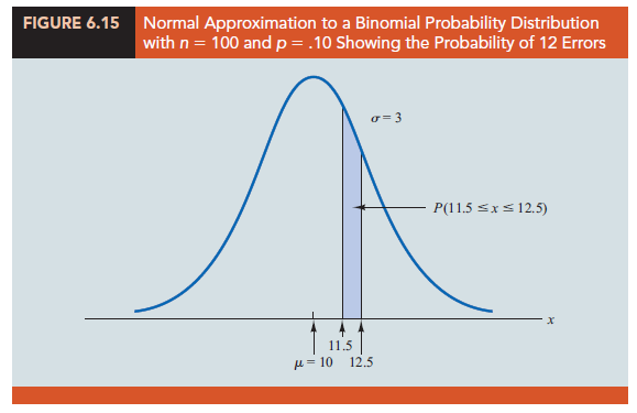
It is introduced because a continuous distribution is being used to approximate a discrete distribution. Thus, P(x = 12) for the discrete binomial distribution is approximated by P(11.5 < x < 12.5) for the continuous normal distribution.

Converting to the standard normal distribution to compute P(11.5 < x < 12.5), we have

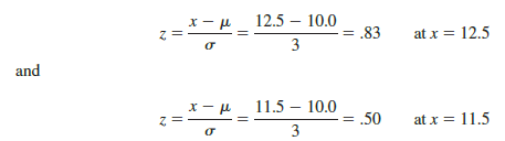
Using the standard normal probability table, we find that the area under the curve (in Fig­ure 6.15) to the left of 12.5 is .7967. Similarly, the area under the curve to the left of 11.5 is .6915. Therefore, the area between 11.5 and 12.5 is .7967 – .6915 = .1052. The normal approximation to the probability of 12 successes in 100 trials is .1052.

For another illustration, suppose we want to compute the probability of 13 or fewer er­rors in the sample of 100 invoices. Figure 6.16 shows the area under the normal curve that approximates this probability. Note that the use of the continuity correction factor results in the value of 13.5 being used to compute the desired probability. The z value corresponding to x = 13.5 is

The standard normal probability table shows that the area under the standard normal curve to the left of z = 1.17 is .8790. The area under the normal curve approximating the probab­ility of 13 or fewer errors is given by the shaded portion of the graph in Figure 6.16.

Source:  Anderson David R., Sweeney Dennis J., Williams Thomas A. (2019), Statistics for Business & Economics, Cengage Learning; 14th edition.