Importing Data from Other Programs to Stata

Previous sections illustrated how to enter and edit data using the Data Editor. If our original data reside in an appropriately formatted spreadsheet, we just can copy and paste blocks of data from the spreadsheet into the empty Data Editor. Alternatively, Stata can import data from Excel spreadsheets directly through menu selections

File > Import > Excel spreadsheet (*.xls; *.xlsx)

or the import excel command. In the simplest case, we could import the first sheet in a spreadsheet file named snowfall.xls by typing the command

. import excel using C:\data\snowfall.xls, clear

But spreadsheets often contain titles, notes, subtables, multiple sheets, graphs or other features that complicate the process of reading them as data. To restrict the import operation to a particular range of cells, use a cellrange() option. The sheet() option can specify what sheet within the spreadsheet to import. A firstrow option tells Stata the first row of these cells contain variables names. For example, in spreadsheet snowfall.xls the first sheet, named “Berlin”, contains historical snowfall records for the town of Berlin, New Hampshire, as discussed in Hamilton et al. (2003). The data of interest reside in cells A5 through O56. Row 4 contains variable names.

. import excel using C:\data\snowfall.xls, sheet(“Berlin”) cellrange(a4:o56) firstrow clear

Although the import excel feature is fairly robust, some preparation of the Excel spreadsheet may speed the transition to an analyzable Stata dataset. For example, if there are variable names in the spreadsheet these should meet Stata criteria such as starting with a letter or underscore, and have no embedded blanks. Missing values should be replaced with blanks or numerical codes, and non-numeric characters removed from cells in columns meant to represent numerical variables.

Stata automatically decides whether each data column represents a numeric or string variable. If there are non-numeric values in a column, Stata takes that column to be a string variable, for which statistical calculations such as means and correlations will not be possible. If most of the values really are numeric, we could generate a new numerical version of that variable (with its actual string values coded as missing) using the real() function.

. generate newvar = real(oldvar)

Similar care is needed when we copy and paste from a spreadsheet into the Data Editor. Before selecting the block of data to copy, editing of the spreadsheet might be needed. One nice trick is to insert a row of variable names right above the top row of data in our spreadsheet. Then copy the row of names along with the rest of the data, and use Paste Special with Treat first row as variable names to place all of this information into an empty Data Editor.

The spreadsheet and Data Editor methods are quick and easy, but for larger projects it is important to have tools that work directly with computer files created by other statistical programs such as SAS or SPSS. SAS XPORT files can be imported through Stata menu choices

File > Import > SAS XPORT

or the import sasxport command. Other data formats can be read through the intermediate form of text files, or translated directly by a special third-party program.

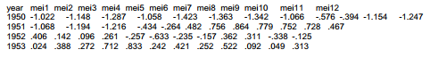
We can illustrate text file methods with another climate-themed time series. El Nino-Southern Oscillation (ENSO) is a quasi-periodic climate pattern centered in the tropical Pacific Ocean but affecting other regions as well. The Multivariate ENSO Index (MEI) combines six observed variables describing tropical Pacific conditions (sea-level pressure, zonal and meridional surface winds, sea surface and surface air temperature, and cloudiness) into a single indicator for ENSO. Text file MEI.raw contains monthly values of MEI from January 1950 through December 2011. These are tab-separated values, a common format for text files written by spreadsheets. The first row of the text file contains a list of variable names: meil for January MEI, mei2 for February, and so forth (actually the “January” MEI value represents December-January, and February represents January-February, etc.). The first few rows of the text file look like this:

We can read these data into Stata using the insheet command, with options to specify that values are tab-separated, and the first row contains variable names. After reading in the raw data we save them as a Stata-format file named MEIO.dta, which will be used again later.

With a comma option instead of tab, insheet could read a text file of comma-separated values, which are another common spreadsheet output format. Text files can be read through Stata menus as well. Explore Data > Import to see the options available.

The examples so far assumed that raw data values are separated by commas, tabs or other known delimiters (which could be replaced with commas or tabs). A different arrangement calledfixed- column format has values that are not necessarily delimited at all, but do occupy predefined column positions. The infix command can read such files. In the command syntax itself, or in a data dictionary existing in a separate file or as the first part of the data file, we have to specify exactly how the columns should be read.

Here is a simple example. Data exist in a text (ASCII) file named nfresour.raw:

These data concern natural resource production in Newfoundland. The four variables occupy fixed column positions: columns 1-4 are the years (1986…1991); columns 5-8 measure forestry production in thousands of cubic meters (2408…missing); columns 9-14 measure mine production in thousands of dollars (764,169…793,000); and columns 15-18 are the consumer price index relative to 1986 (1000…1262). Notice that in fixed-column format, unlike whitespace or tab-delimited files, blanks indicate missing values, and the raw data contain no decimal points. To read nfresour.raw into Stata, we specify each variable’s column position:

More complicated fixed-column formats might require a data dictionary. Data dictionaries can be straightforward, but they offer many possible choices. Type help import to see an outline of these commands. For more examples and explanation, consult the User’s Guide and reference manuals. Stata also can load, write, or view data from ODBC (Open Database Connectivity) sources; see help odbc.

What if we need to export data from Stata to some other, non-ODBC program? export excel and export sasxport commands, or corresponding menu selections from

File > Export > Excel spreadsheet (*.xls; *.xlsx) File > Export > SAS XPORT

will write Excel spreadsheets or SAS XPORT files. The outsheet and outfile commands (or Data > Export ) can write text files in several different formats. Another very quick possibility is to copy your data from Stata’s Data Editor or Data Browser and paste this directly into a spreadsheet such as Excel. Often the best option, however, is to transfer data directly between the specialized system files saved by various spreadsheet, database or statistical programs. Some third-party programs perform such translations. Stat/Transfer, for example, will transfer data across many different formats including dBASE, Excel, FoxPro, Gauss, JMP, MATLAB, Minitab, OSIRIS, Paradox, R, S-Plus, SAS, SPSS, SYSTAT and Stata. Even large datasets hundreds of megabytes in size can be translated or excerpted quickly with this program. It is available through StataCorp (www.stata.com) or from its maker, Circle Systems (www.stattransfer.com). Transfer programs prove indispensable for analysts working in multi­program environments or exchanging data with colleagues.

One distinguishing feature of Stata is worth mentioning here. Stata datasets saved on one Stata platform (whether Windows, Mac or Unix) can be read without translation by Stata on any of the other platforms. To make a data file that can be read by an earlier version of Stata on any of these platforms, use the saveold command instead of save, or select

Save As > Save as type > Stata 9/10 Data from the menus.

Source: Hamilton Lawrence C. (2012), Statistics with STATA: Version 12, Cengage Learning; 8th edition.