Managing Publication Bias of Meta-Analysis

In this section, I describe six approaches to managing publication bias within meta-analysis. I also illustrate some of these approaches through the example meta-analysis I have used throughout this book: a review of 22 studies report­ing associations between relational aggression and peer rejection among chil­dren and adolescents. In Chapter 8, I presented results of a fixed-effects³ analysis of these studies indicating a mean r = .368 (SE = .0118; Z = 32.70, p < .001; 95% confidence interval = .348 to .388). When using this example in this section, I evaluate the extent to which this conclusion about the mean association is threatened by potential publication bias.

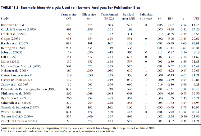
Table 11.1 displays these 22 studies. The first five columns of this table are the citation, sample size, untransformed effect size (r), transformed effect size (Z_r), and standard error of the transformed effect size (SE). The remain­ing columns contain information that I explain when using these data to illustrate methods of evaluating publication bias.

1. Moderator Analyses

One of the best methods to evaluate the potential impact of publication bias is to include unpublished studies in the meta-analysis and empirically evalu­ate whether these studies yield smaller effect sizes than published studies. In the simplest case, this involves evaluating the moderation of effect sizes (Chapter 10) by the dichotomous variable, published versus unpublished study. Two caveats to this approach merit consideration. First, it is necessary to make sure that the meta-analysis includes a sufficient number of unpub­lished studies to draw reliable conclusions about potential differences. Sec­ond, it is important to consider other features on which published versus unpublished studies might differ, such as the quality of the methodology (e.g., internal validity of an experimental design) and measures (e.g., use of reliable vs. unreliable scales). You should control for such differences when comparing published and unpublished studies.

A more elaborate variant of this sort of moderator analysis is to code more detailed variables regarding publication status. For instance, you might code a more continuous publication quality variable (e.g., distinguishing unpublished data, dissertations, conference presentations, low-tier journal articles, and top-tier journal articles, if this captures a meaningful contin­uum within your field). You might also code whether the effect size of inter­est is a central versus peripheral result in the study; for instance, Card et al. (2008) considered whether terms such as “gender” or “sex” appeared in titles of works reporting gender differences in childhood aggression.

Regardless of which variables you code, the key question is whether these variables are related to the effect sizes found in the studies (i.e., whether these act as moderators). If you find no differences between published and unpub­lished studies (or absence of moderating effects of other variables such as publication quality and centrality), and there is adequate power to detect such moderation, then it is safe to conclude that there is no evidence of publication bias within this area. If differences do exist, you have the choice of either (1) interpreting results of published and unpublished studies separately, or (2) performing corrections for publication bias described below (Section 11.3).

To illustrate this approach to evaluating publication bias, I consider one approach I have described: moderation by the categorical moderator “pub­lished.” This categorical variable is shown in the sixth column of Table 11.1 and is coded as 1 for studies that were published (k = 15) and 0 for unpub­lished studies (k = 7). Notice that this comparison is possible only because I included unpublished studies in this meta-analysis and the search was thor­ough enough to obtain a sufficient number of unpublished studies for com­parison. Moderator analyses (Chapter 9) indicated a significant difference between published and unpublished studies (Qb_et_ween(1df) = 77.47, p < .001). In the absence of publication bias, I would not expect this moderator effect, so its presence is worrisome. When I inspect the mean effects sizes within each group, I find that the unpublished studies yield higher associations (r = .51) than the published studies (r = .31). This runs counter to the possibility that nonsignificant/low effect size studies are less likely to be published; if there is a bias, it appears that studies finding large effect sizes are less likely to be published and therefore any publication bias might serve to diminish the effect size I find in this meta-analysis. However, based on my knowledge of the field (and conversations with other experts about this finding), I see no apparent reason why there would be a bias against publishing studies find­ing strong positive correlations. I consider this finding further in light of my other findings regarding potential publication bias below.

2. Funnel Plots

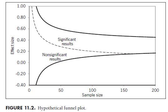
Funnel plots represent a graphical way to evaluate publication bias (Light & Pillemer, 1984; see Sterne, Becker, & Egger, 2005). The funnel plots are simply a scatterplot of the effect sizes found in studies relative to their sample size (with some variants on this general pattern). In other words, you would simply plot points for each study denoting their effect size relative to their sample size. Figure 11.2 shows a hypothetical outline of a funnel plot, with the effect size Z_r on the y-axis and sample size (N) on the x-axis.⁴ Specifi­cally, the solid lines within this figure represent the 95% confidence interval of effect sizes centered around r = .30 (Z_r = .31; see below) at various sample sizes⁵; if you plot study effect sizes and sample sizes from a sample with this mean effect size, then most (95%) of the points should fall within the area between these solid lines. On the left, you can see that there is considerably larger expectable variability in effect sizes with small sample sizes; conceptu­ally, you expect that studies with small samples will yield a wider range of effect sizes due to random-sampling variability. In contrast, as sample sizes increase, the expectable variability in effect sizes becomes smaller (i.e., the standard errors become smaller), and so the funnel plot shows a narrower distribution of effect sizes at the right of Figure 11.2. Evaluation of publica­tion bias using funnel plots involves visually inspecting these plots to ensure symmetry and this general triangular shape.

Let’s now consider how publication bias would affect the shape of this funnel plot. Note the dashed line passing through the funnel plot. This line represents the magnitude of effect size needed to achieve statistical signifi-cance (p < .05) at various sample sizes. The area above and to the right of this dashed line would denote studies finding significant effects, whereas the area below and to the left of it would contain studies that do not yield significant effects. If publication bias exists, then you would see few points (i.e., few studies in your meta-analysis) that fall within this nonsignificant region. This would cause your funnel plot to look asymmetric, with small sample studies finding large effects present but small studies finding small effects absent.

Publication bias is not the only possible cause of asymmetric funnel plots. If studies with smaller samples are expected to yield stronger effect sizes (e.g., studies of intervention effectiveness might be able to devote more resources to a smaller number of participants), then this asymmetry may not be due to publication bias. In these situations, you would ideally code the presumed difference between small and large sample studies (e.g., amount of time or resources devoted to participants) and control for this⁶ before creat­ing the funnel plot.

Several variants of the axes used for funnel plots exist. You might con­sider alternative choices of scale on the effect size axis. I recommend relying on effect sizes that are roughly normally distributed around a population effect size, such as Fisher’s transformation of the correlation (Z_r), Hedges’s g, or the natural log of the odds ratio (see Chapter 5). Using normally distrib­uted effect sizes, as opposed to non-normal effect sizes (e.g., r or o) allows for better examination of the symmetry of funnel plots. Similarly, you have choices of how to scale the sample size axis. Here, you might consider using the natural log of sample size, which aids interpretation if some studies use extremely large samples that compress the rest of the studies into a narrow range of the funnel plot. Other choices include choosing standard errors, their inverse (precision), or weights (1 / SE²) on this axis; this option is rec­ommended when you are analyzing log odds ratios (Sterne et al., 2005) and might also be useful when the standard error is not perfectly related to sam­ple size (e.g., when you correct for artifacts). I see no problem with examin­ing multiple funnel plots when evaluating publication bias. Given that the examination of funnel plots is somewhat subjective, I believe that examining these plots from several perspectives (i.e., several different choices of axis scaling) is valuable in obtaining a complete picture about the possibility of publication bias.

To illustrate the use of funnel plots—as well as the major challenges in their use—I have plotted the 22 studies from Table 11.1 in Figure 11.3.

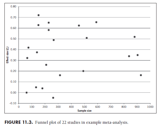
I created this plot simply by constructing a scatterplot with transformed effect size (fourth column in Table 11.1) on the vertical axis and sample size (second column in Table 11.1) on the horizontal axis. My inspection of this plot leads me to conclude that there is no noticeable asymmetry or sparse representation of studies in the low effect size—low sample size area (i.e., where results would be nonsignificant). I also perceive that the effect sizes tend to become less discrepant with larger sample sizes—that is, that the plot becomes more vertically narrow from the left to the right. However, you might not agree with these conclusions. This raises the challenge of using funnel plots—that the interpretations you take from these plots are neces­sarily subjective. This subjectivity is especially prominent when the number of studies in your meta-analysis is small; in my example with just 22 studies, it is extremely difficult to draw indisputable conclusions.

3. Regression Analysis

Extending the logic of funnel plots, you can more formally test for asymme­try by regressing effect sizes onto sample sizes. The presence of an associa­tion between effect sizes and sample sizes is similar to an asymmetric funnel plot in suggesting publication bias. In the case of a positive mean effect size, publication bias will be evident when studies with small sample sizes yield larger effect size estimates than studies with larger samples; this situation would produce a negative association between sample size and effect size. In contrast, when the mean effect size is negative, then publication bias will be indicated by a positive association (because studies with small samples yield stronger negative effect size estimates than studies with larger samples). The absence of an association, given adequate statistical power to detect one, par­allels the symmetry of the funnel plot in suggesting an absence of publication bias.

Despite the conceptual simplicity of this approach, recommended prac­tices (see Sterne & Egger, 2005) build on this conceptual approach but make it somewhat more complex. Specifically, two variants of this regression approach are commonly employed. The first involves considering an adjusted rank correlation between studies’ effect sizes and standard errors (for details, see Begg, 1994; Sterne & Egger, 2005). To perform this analysis, you use the following two equations to compute, for each study i, the variance of the study’s effect size from the mean effect size (v*) and the standardized effect size for study (ES*):

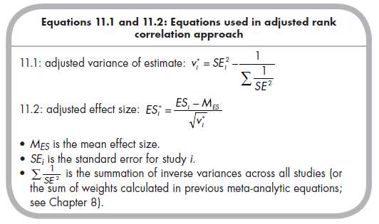
After computing these variables, you then estimate Kendall’s rank cor­relation between v* and ES*. A significant correlation indicates funnel plot asymmetry, which may suggest publication bias. An absence of correlation contraindicates publication bias, if power is adequate.

A comparable approach is Egger’s linear regression, in which you regress the standard normal deviate of the effect size of each study from zero (i.e., for study i, Zi = ESj / SE*) onto the precision (the inverse of the SE, or 1/ SE*): Zi = Bq + Biprecisioni + ei. Somewhat counterintuitively, the slope (Bi) repre­sents the average effect size (because both the DV and predictor have SE in their denominator, this is similar to regressing the ES onto a constant, which yields the mean ES). The intercept (Bq, which is similar to regressing the ES onto the SE) is expected to be zero, and a nonzero intercept (the signifi­cance of which can be evaluated using common statistical software) indicates asymmetry in the funnel plot, or the possibility of publication bias.

These regression approaches to evaluating funnel plot asymmetry (which can be indicative of publication bias) are advantageous over visual inspection of funnel plots in that they reduce subjectivity by providing results that can be evaluated in terms of statistical significance. However, these regression approaches depend on the absence of statistically significant results to con­clude an absence of publication bias (which is typically what you hope to demonstrate). Therefore, their utility depends on adequate statistical power to detect asymmetry. Although the number of simulation studies are lim­ited (for a review, see Sterne & Egger, 2005), preliminary guidelines for the number of studies needed to ensure adequate power can be provided. When
publication bias is severe (and targeting 80% power), at least 17 studies are needed with Egger’s linear regression approach, and you should have at least 40 studies for the rank correlation method (note that this is an extrapolation from previous simulations and should be interpreted with caution). When publication bias is moderate, you should have at least 50 to 60 studies for Egger’s linear regressions and at least 150 studies for the rank correlation approaches. However, I emphasize again that these numbers are extrapolated well beyond previous studies and should be viewed with extreme caution until further studies investigate the statistical power of these approaches.

Considering again the 22 studies of my example meta-analysis, I eval­uated the association between effect size and sample size using both the adjusted rank correlation approach and Egger’s linear regression approach. Columns seven and eight in Table 11.1 show the two transformed variables for the former approach, and computation of Kendall’s rank correlation yielded a nonsignificant value of -.07 (p = .67). Similarly, Egger’s regression of the val­ues in the ninth column onto those in the tenth was nonsignificant (p = .62). I would interpret both results as failing to indicate evidence of publication bias. However, I should be aware that my use of just 22 studies means that I only have adequate power to detect severe publication bias using Egger’s linear regression approach, and I do not have adequate power with the rank correlation method.

4. Failsafe N

4.1. Definition and Computation

Failsafe numbers (failsafe N) help us evaluate the robustness of a meta­analytic finding to the existence of excluded studies. Specifically, the failsafe number is the number of excluded studies, all averaging an effect size of zero, that would have to exist for their inclusion in the meta-analysis to lower the average effect size to a nonsignificant level.⁷ This number, introduced by Rosenthal (1979) as an approach to dealing with the “file drawer problem,” also can be thought of as the number of excluded studies (all with average effect sizes equal to zero) that would have to be filed away before you would conclude that no effect actually exists (if the meta-analyst had been able to analyze results from all studies conducted). If this number is large enough, you conclude that it is unlikely that you could have missed so many stud­ies (that researchers’ file drawers are unlikely to be filled with so many null results), and therefore that this conclusion of the meta-analysis is robust to this threat.

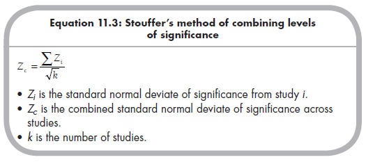
The computation of a failsafe number begins with the logic of an older method of combining research results, known as Stouffer’s or the sum-of-Zs method (for an overview of these earlier methods of combining results, see Rosenthal, 1978). This method involves computing the significance level of the effect from each study (the one-tailed p value), converting this to a stan­dard normal deviate (Zj, with positive values denoting effects in expected direction), and then combining these Zs across the k studies to obtain an overall combined significance (given by standardized normal deviate, Z_c):

Failsafe N extends this approach by asking the question, How many studies could be added to those in the meta-analysis (going from k to k + N in the denominator term of Equation 11.4), all with zero effect sizes (Zs = 0, so the numerator term does not change), before the significance level drops to some threshold value (e.g., Z_c = Z_a = 1.645 for one-tailed p = .05)? The equa­tion can be rearranged to yield the computation formula for failsafe N:

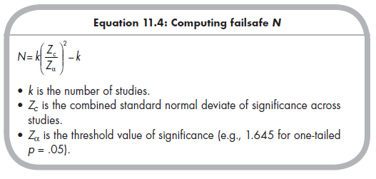
Examination of these equations makes clear the two factors that impact the failsafe N. The first is the level of statistical significance (Z_c) yielded from the included results (which is a function of effect size and sample size of the study); the larger this value, the larger the failsafe N. The second factor is the number of included studies, k. Increasing numbers of included studies results in increasing failsafe Ns (because the first occurrence of k in Equa­tion 11.5 is multiplied by a ratio greater than 1 [when results are significant], this offsets the subtraction by k). This makes intuitive sense: Meta-analyses finding a low p value (e.g., far below .05) from results from a large number of studies need more excluded, null results to threaten the findings, whereas meta-analyses with results closer to what can be consider a “critical” p value (e.g., just below .05) from a small number of studies could be threatened by a small number of excluded studies.

How large should failsafe N be before you conclude that results are robust to the file drawer problem? Despite the widespread use of this approach over about 30 years, no one has provided a statistically well-founded answer. Rosenthal’s (1979) initial suggestion was for a tolerance level (i.e., adequately high failsafe N) equal to 5 k + 10, and this initial suggestion seems to have been the standard most commonly applied since. Rosenthal (1979) noted what is a plausible number of studies filed away likely depends on the area of research, but no one has further investigated this speculation. At the moment, the 5k + 10 is a reasonable standard, though I hope that future work will improve on (or at least provide more justification for) this value.

4.2. Criticisms

Despite their widespread use, failsafe numbers have been criticized in sev­eral ways (see Becker, 2005). Although these criticisms are valuable in point­ing out the limits of using failsafe N exclusively, I do not believe that they imply that you should not use this approach. Next, I briefly outline the major criticisms against failsafe N and suggest considerations that temper these critiques.

One criticism is of the premise of computing the number of studies with null results. The critics argue that other possibilities could be considered, such as studies in the opposite direction as those found in the meta-analysis. It is true that any alternative effect size could be chosen; but it seems that selection of null results (i.e., those with effect sizes close to 0), which are the studies expected to be suppressed under most conceptualizations of publica­tion bias, represents the most appropriate single value to consider.

A second criticism of the failsafe number is that it does not consider the sample sizes of the excluded studies. Sample sizes of included studies are indirectly considered in that larger samples sizes yield larger Z;s than smaller studies, given the same effect size. In contrast, excluded studies are assumed to have effect sizes of zero and therefore Zs equal to zero regard­less of sample size. So, the failsafe number would not differentiate between excluded studies with sample sizes equal to 10 versus 10,000. I believe this is a fair critique of failsafe N, though the impact depends on excluded studies with zero effect sizes (on average) having larger sample sizes than included studies. This seems unlikely given the previous consideration of publication bias and funnel plots. If there is a bias, I would expect that excluded studies are primarily those with small (e.g., near zero) effect sizes and small sample sizes (however, I acknowledge that I am unaware of empirical support for this expectation).

A third criticism involves the failure of failsafe N to model heterogeneity among obtained results. In other words, the Stouffer method of obtaining the overall significance (Z_c) among included studies, which is then used in the computation of failsafe N, makes no allowance for whether these studies are homogeneous (centered around a mean effect size with no more deviation than expected by sampling error) or heterogeneous (deviation around mean effect size is greater than expected by sampling error alone; see Chapter 10). This is a valid criticism that should be kept in mind when interpreting fail­safe N. I especially recommend against using failsafe N when heterogeneity necessitates the use of random-effects models (Chapter 9).

A final criticism of Rosenthal’s (1979) failsafe N is the focus on statisti­cal significance. As I have discussed throughout this book, one advantage of meta-analysis is a focus on effect sizes; a number that indicates the number of excluded studies that would reduce your results to nonsignificance does not tell you how these might affect your results in terms of effect size. For this, an alternative failsafe number can be considered, which I describe next.

4.3. An Effect Size Failsafe N

An alternative approach that focuses on effect sizes was proposed by Orwin (1983; see also Becker, 2005). Using this approach, you select an effect size⁸ (smaller than that obtained in the meta-analysis of sampled studies) that rep­resents the smallest meaningful effect size (either from guidelines such as r = ±.10 for a small effect size, or preferably an effect size that is meaningful in the context of the research). This value is denoted as ES_mj_n.⁹ You then com­ pute a failsafe number (Nes) from the meta-analytically combined average effect size (E5m) from the k included studies using:

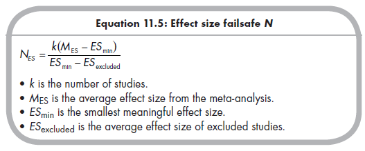
The denominator of this equation introduces an additional term that I have not yet described, ES_excj_ud_ed- This represents the expected (i.e., speci­fied by the meta-analyst) average effect size of excluded studies. A reasonable choice, paralleling the assumption of Rosenthal’s (1979) approach, might be zero. In this case, the failsafe number (Nes) would tell us how many excluded studies with an average effect size of zero would have to exist before the true effect size would be reduced to the smallest meaningful effect size (E5_mj_n). Although this is likely a good choice for many situations, the flexibility to specify alternative effect sizes of excluded studies addresses the first criti­cism of traditional approaches described above.

Although this approach to failsafe N based on minimum effect size alle­viates two critiques of Rosenthal’s original approach, it is still subject to the other two criticisms. First, this approach still assumes that the excluded studies have the same average sample size as included studies. I believe that this results in a conservative bias in most situations; if the excluded studies tend to have smaller samples than the included studies, then the failsafe N is smaller than necessary. Second, this approach also does not model het­erogeneity, and therefore is not informative when you find significant het­erogeneity and rely on random-effects models. A third limitation, unique to this approach, is that there do not exist solid guidelines for determining how large the failsafe number should be before you conclude that results are robust to the file drawer problem. I suspect that this number is smaller than Rosenthal’s (1979) 5k + 10 rule, but more precise numbers have not been developed.

To illustrate computation of these failsafe numbers, I again consider the example meta-analysis of Table 11.1. Summing the Zs (not the Z_rs) across the 22 studies yields 127.93, from which I compute Z_c = 127.93 / V22 = 27.27. To compute Rosenthal’s (1979) failsafe number of studies with effect sizes of zero needed to reduce the relational aggression with rejection association to nonsignificance, I apply Equation 11.4:

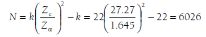
This means that there could exist up to 6,026 studies, with an average cor­relation of 0, before my conclusion of a significant association is threatened. This is greater than the value recommended by Rosenthal (1979) (i.e., 5k + 10 = 5*22 + 10 = 120), so I would conclude that my conclusion of an association between relational aggression and rejection is robust to the file drawer prob­lem. However, it is more satisfying to discuss the robustness of the magni­tude, rather than just the significance of this association, so I also use Orwin’s (1983) approach of Equation 11.5. Under the assumption that excluded stud­ies have effect sizes of 0 (i.e., in Equation 11.5, ES_excl_uq_ed = 0), I find that 5 excluded studies could reduce the average correlation to .30, 19 could reduce it to .20, and 59 would be needed to reduce it to .10. Although there are no established guidelines for Orwin’s failsafe numbers, it seems reasonable to conclude that it is plausible that the effect size could be less than a medium correlation (i.e., less than the standard of r = ±.30) but perhaps implausible that the effect size could be less than a small correlation (i.e., less than the standard of r = ±.10).

5. Trim and Fill

The trim and fill method is a method of correcting for publication bias (see Duval, 2005) that involves a two-step iterative procedure. The conceptual rationale for this method is illustrated by considering the implications of publication bias on funnel plots (recall that the corner of the funnel denoting studies with small sample sizes and small effect sizes is underrepresented), which causes bias in estimating both the mean effect size and the heteroge­neity around this effect size. The trim and fill approach uses a two-step cor­rection that attempts to provide more accurate estimates of both mean and spread in effect sizes.

The first step of this approach is to temporarily “trim” studies contribut­ing to funnel plot asymmetry. Considering Figure 11.2 (in which the funnel plot is expected to be asymmetric in having more studies in the upper left section than the lower left section when there is publication bias), this trim­ ming involves temporarily removing studies until you obtain a symmetric funnel plot (often shaped like a bar in the vertical middle of this plot). You then estimate an unbiased mean effect size from the remaining studies for use in the second step.

The second step involves reinstating the previously trimmed studies (resulting in the original asymmetric funnel plot) and then imputing studies in the underrepresented section (lower left of Figure 11.2) until you obtain a symmetric funnel plot. This symmetric funnel plot allows for accurate esti­mation of both the mean and heterogeneity (or between-study variance) of effect sizes. This two-step process is repeated several times until you reach a convergence criterion (in which trimming and filling produce little change to estimates).

As you might expect, this is not an approach performed by hand, and the exact statistical details of trimming and filling are more complex than I have presented here (for details, see Duval, 2005). Fortunately, this approach is included in some software packages for meta-analysis (this represents an exception to my general statement that meta-analysis can be conducted by hand or with a simple spreadsheet program, though you could likely program this approach into traditional software packages). There also exist variations depending on modeling of between-study variability beyond sampling fluctu­ation (random- versus fixed-effects) and choice of estimation method. These methods have not yet been fully resolved.

Despite the need for specialized software and some unresolved statisti­cal issues, the trim and fill method represents a useful way to correct for potential publication bias. Importantly, this method is not to be used as the primary reporting of results of a meta-analysis. In other words, you should not impute study values, analyze the resulting dataset including these values, and report the results as if this was what was “found” in the meta-analysis. Instead, you should compute results using the trim and fill method for com­parison to those found from the studies actually obtained. If the estimates are comparable, then you conclude that the original results are robust to publica­tion bias, whereas discrepancies suggest that the obtained studies produced biased results.

6. Weighted Selection Approaches

An additional method of managing publication bias is through selection method approaches (Hedges & Vevea, 2005), also called weighted distribu­tion theory corrections (Begg, 1994). These methods are complex, and I do not attempt to fully describe them fully here (see Hedges & Vevea, 2005). The central concept of these approaches is to construct a distribution of inclu­sion likelihood (i.e., a selection model) that is used for weighting the results obtained. Specifically, studies with characteristics that are related to lower likelihood of inclusion are given more weight than studies with characteris­tics related to higher likelihood of inclusion.

This distribution of inclusion likelihood is based on characteristics of studies that are believed to be related to inclusion in the meta-analysis. For example, you might expect the likelihood to be related to the level of sta­tistical significance, such that studies finding significant results are more likely to be included than those that do not. Because it is usually difficult to empirically derive values for this likelihood distribution, the most com­mon practice is to base these on a priori models. A variety of models have been suggested (see Begg, 1994; Hedges & Vevea, 2005), including models that propose equal likelihood for studies with p < .05 and then a gradually declining likelihood, as well as models that consist of steps corresponding to diminished likelihood at ps that are psychologically salient (e.g., ps = .01, .05, .10). Other models focus more on effect sizes, sometimes in combination with standard errors. Your choice of one of these models should be guided by the underlying selection process that you believe is operating, though this deci­sion can be difficult to make in the absence of field-specific information. It is also necessary for these approaches to be applied within a meta-analysis with a large number of studies. In sum, this weighted selection approach appears promising, but some important practical issues need to be resolved before they can be widely used.

Source: Card Noel A. (2015), Applied Meta-Analysis for Social Science Research, The Guilford Press; Annotated edition.