Understanding and Predicting the Effects of Changing Market Conditions

So far, our discussion of supply and demand has been largely qualitative. To use supply and demand curves to analyze and predict the effects of changing market conditions, we must begin attaching numbers to them. For example, to see how a 50-percent reduction in the supply of Brazilian coffee may affect the world price of coffee, we must determine actual supply and demand curves and then calculate the shifts in those curves and the resulting changes in price.

In this section, we will see how to do simple “back of the envelope” calcula- tions with linear supply and demand curves. Although they are often approxi- mations of more complex curves, we use linear curves because they are easier to work with. It may come as a surprise, but one can do some informative economic analyses on the back of a small envelope with a pencil and a pocket calculator.

First, we must learn how to “fit” linear demand and supply curves to market data. (By this we do not mean statistical fitting in the sense of linear regression or other statistical techniques, which we will discuss later in the book.) Suppose we have two sets of numbers for a particular market: The first set consists of the price and quantity that generally prevail in the market (i.e., the price and quantity that prevail “on average,” when the market is in equilibrium or when market conditions are “normal”). We call these numbers the equilibrium price and quantity and denote them by P* and Q*. The second set consists of the price elasticities of supply and demand for the market (at or near the equilibrium), which we denote by ES and ED, as before.

These numbers may come from a statistical study done by someone else; they may be numbers that we simply think are reasonable; or they may be numbers that we want to try out on a “what if” basis. Our goal is to write down the sup-ply and demand curves that fit (i.e., are consistent with) these numbers. We can then determine numerically how a change in a variable such as GDP, the price of another good, or some cost of production will cause supply or demand to shift and thereby affect market price and quantity.

Let’s begin with the linear curves shown in Figure 2.19. We can write these curves algebraically as follows:

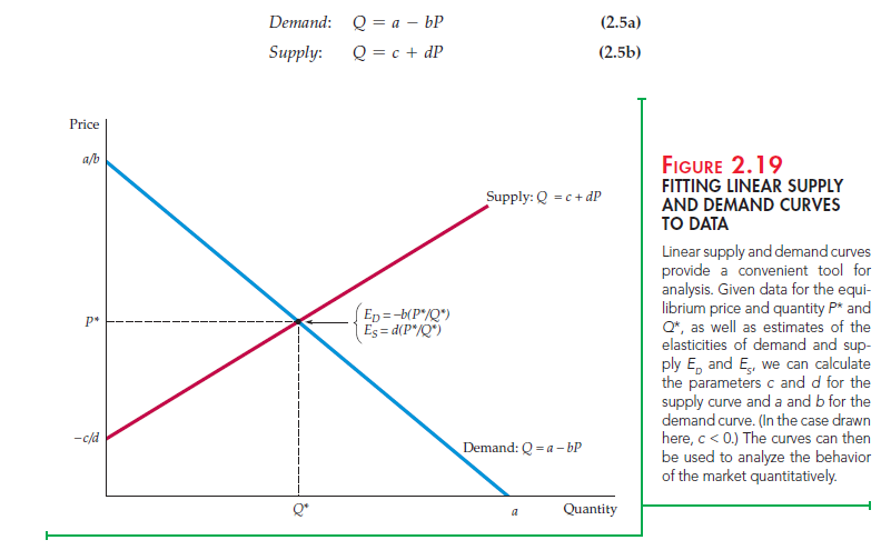
Our problem is to choose numbers for the constants a, b, c, and d. This is done, for supply and for demand, in a two-step procedure:

• Step 1:Recall that each price elasticity, whether of supply or demand, can be written as

E = (P/Q)(AQ/AP)

where AQ/ AP is the change in quantity demanded or supplied resulting from a small change in price. For linear curves, AQ/ AP is constant. From equations (2.5a) and (2.5b), we see that AQ/AP = d for supply and AQ/AP = -b for demand. Now, let’s substitute these values for AQ/ AP into the elasticity formula:

Demand: E_D = – b(P*/Q*)                                             (2.6a)

Supply:     E_S = d(P*/Q*)                                              (2.6b)

where P* and Q* are the equilibrium price and quantity for which we have data and to which we want to fit the curves. Because we have numbers for E_S, E_d, P*, and Q*, we can substitute these numbers in equations (2.6a) and (2.6b) and solve for b and d.

• Step 2:Since we now know b and d, we can substitute these numbers, as well as P* and Q*, into equations (2.5a) and (2.5b) and solve for the remaining constants a and c. For example, we can rewrite equation (2.5a) as

a = Q* + bP*

and then use our data for Q* and P*, together with the number we calculated in Step 1 for b, to obtain a.

Let’s apply this procedure to a specific example: long-run supply and demand for the world copper market. The relevant numbers for this market are as follows:

Quantity Q* = 18 million metric tons per year (mmt/yr)

Price P* = $3.00 per pound Elasticity of suppy E_S = 1.5 Elasticity of demand E_D = — 0.5.

(The price of copper has fluctuated during the past few decades between $0.60 and more than $4.00, but $3.00 is a reasonable average price for 2008-2011).

We begin with the supply curve equation (2.5b) and use our two-step proce­dure to calculate numbers for c and d. The long-run price elasticity of supply is 1.5, P* = $3.00, and Q* = 18.

• Step 1:Substitute these numbers in equation (2.6b) to determine d:

1.5 = d(3/18) = d/6

so that d = (1.5)(6) = 9.

• Step 2: Substitute this number for d, together with the numbers for P* and Q*, into equation (2.5b) to determine c:

18 = c + (9)(3.00) = c + 27

so that c = 18 – 27 = -9. We now know c and d, so we can write our supply curve:

Supply:   Q = — 9 + 9P

We can now follow the same steps for the demand curve equation (2.5a). An estimate for the long-run elasticity of demand is -0.5.^[1] First, substitute this number, as well as the values for P* and Q*, into equation (2.6a) to determine b:

– 0.5 = – b(3/18) = – b/6

so that b = (0.5)(6) = 3. Second, substitute this value for b and the values for P* and Q* in equation (2.5a) to determine a:

18 = a = (3)(3) = a – 9

so that a = 18 + 9 = 27. Thus, our demand curve is:

Demand:    Q = 27 — 3P

To check that we have not made a mistake, let’s set the quantity supplied equal to the quantity demanded and calculate the resulting equilibrium price:

Supply = — 9 + 9P = 27 — 3P = Demand
9P + 3P = 27 + 9

or P = 36/12 = 3.00, which is indeed the equilibrium price with which we began.

Although we have written supply and demand so that they depend only on price, they could easily depend on other variables as well. Demand, for example, might depend on income as well as price. We would then write demand as

Q = a — bP + fI                                                      (2.7)

where I is an index of the aggregate income or GDP. For example, I might equal 1.0 in a base year and then rise or fall to reflect percentage increases or decreases in aggregate income.

For our copper market example, a reasonable estimate for the long-run income elasticity of demand is 1.3. For the linear demand curve (2.7), we can then calculate f by using the formula for the income elasticity of demand: E = (I/Q)(AQ/AI). Taking the base value of I as 1.0, we have

1.3 = (1.0/18)( f).

Thus f = (1.3)(18)/(1.0) = 23.4. Finally, substituting the values b = 3, f = 23.4, P* = 3.00, and Q* = 18 into equation (2.7), we can calculate that a must equal 3.6.

We have seen how to fit linear supply and demand curves to data. Now, to see how these curves can be used to analyze markets, let’s look at Example 2.8, which deals with the behavior of copper prices, and Example 2.9, which concerns the world oil market.

Source: Pindyck Robert, Rubinfeld Daniel (2012), Microeconomics, Pearson, 8th edition.