Binomial Probability Distribution

The binomial probability distribution is a discrete probability distribution that has many applications. It is associated with a multiple-step experiment that we call the binomial experiment.

1. A Binomial Experiment

A binomial experiment exhibits the following four properties.

PROPERTIES OF A BINOMIAL EXPERIMENT

1. 1. The experiment consists of a sequence of n identical trials.
   2. Two outcomes are possible on each trial. We refer to one outcome as a success and the other outcome as a
   3. The probability of a success, denoted by p, does not change from trial to trial. Consequently, the probability of a failure, denoted by 1 – p, does not change from trial to trial.
   4. The trials are independent.

If properties 2, 3, and 4 are present, we say the trials are generated by a Bernoulli process. If, in addition, property 1 is present, we say we have a binomial experiment. Figure 5.2 de­picts one possible sequence of successes and failures for a binomial experiment involving eight trials.

In a binomial experiment, our interest is in the number of successes occurring in the n trials. If we let x denote the number of successes occurring in the n trials, we see that x can assume the values of 0, 1, 2, 3, . . . , n. Because the number of values is finite, x is a discrete random variable. The probability distribution associated with this random variable is called the binomial probability distribution. For example, consider the experiment of tossing a coin five times and on each toss observing whether the coin lands with a head or a tail on its upward face. Suppose we want to count the number of heads appearing over the five tosses. Does this experiment show the properties of a binomial experiment? What is the random variable of interest? Note that:

1. The experiment consists of five identical trials; each trial involves the tossing of one coin.
2. Two outcomes are possible for each trial: a head or a tail. We can designate head a success and tail a failure.
3. The probability of a head and the probability of a tail are the same for each trial, with p = .5 and 1 – p = .5.
4. The trials or tosses are independent because the outcome on any one trial is not affected by what happens on other trials or tosses.

Thus, the properties of a binomial experiment are satisfied. The random variable of interest is x = the number of heads appearing in the five trials. In this case, x can assume the values of 0, 1, 2, 3, 4, or 5.

As another example, consider an insurance salesperson who visits 10 randomly selected families. The outcome associated with each visit is classified as a success if the family purchases an insurance policy and a failure if the family does not. From past experience, the salesperson knows the probability that a randomly selected family will purchase an insurance policy is .10. Checking the properties of a binomial experiment, we observe that:

1. The experiment consists of 10 identical trials; each trial involves contacting one family.
2. Two outcomes are possible on each trial: the family purchases a policy (success) or the family does not purchase a policy (failure).
3. The probabilities of a purchase and a nonpurchase are assumed to be the same for each sales call, with p = .10 and 1 – p = .90.
4. The trials are independent because the families are randomly selected.

Because the four assumptions are satisfied, this example is a binomial experiment. The random variable of interest is the number of sales obtained in contacting the 10 families. In this case, x can assume the values of 0, 1, 2, 3, 4, 5, 6, 7, 8, 9, and 10.

Property 3 of the binomial experiment is called the stationarity assumption and is sometimes confused with property 4, independence of trials. To see how they differ, consider again the case of the salesperson calling on families to sell insurance policies. If, as the day wore on, the salesperson got tired and lost enthusiasm, the probability of success (selling a policy) might drop to .05, for example, by the tenth call. In such a case, property 3 (stationarity) would not be satisfied, and we would not have a binomial experiment. Even if property 4 held—that is, the purchase decisions of each family were made independently—it would not be a binomial experiment if property 3 was not satisfied.

In applications involving binomial experiments, a special mathematical formula, called the binomial probability function, can be used to compute the probability of x successes in the n trials. Using probability concepts introduced in Chapter 4, we will show in the context of an illustrative problem how the formula can be developed.

2. Martin Clothing Store Problem

Let us consider the purchase decisions of the next three customers who enter the Martin Clothing Store. On the basis of past experience, the store manager estimates the probability that any one customer will make a purchase is .30. What is the probability that two of the next three customers will make a purchase?

Using a tree diagram (Figure 5.3), we can see that the experiment of observing the three customers each making a purchase decision has eight possible outcomes. Using S to denote success (a purchase) and F to denote failure (no purchase), we are interested in experimental outcomes involving two successes in the three trials (purchase decisions). Next, let us verify that the experiment involving the sequence of three purchase decisions can be viewed as a binomial experiment. Checking the four requirements for a binomial experiment, we note that:

1. The experiment can be described as a sequence of three identical trials, one trial for each of the three customers who will enter the store.
2. Two outcomes—the customer makes a purchase (success) or the customer does not make a purchase (failure)—are possible for each trial.
3. The probability that the customer will make a purchase (.30) or will not make a purchase (.70) is assumed to be the same for all customers.
4. The purchase decision of each customer is independent of the decisions of the other customers.

Hence, the properties of a binomial experiment are present.

The number of experimental outcomes resulting in exactly x successes in n trials can be computed using the following formula.

Now let us return to the Martin Clothing Store experiment involving three customer purchase decisions. Equation (5.10) can be used to determine the number of experimental outcomes involving two purchases; that is, the number of ways of obtaining x = 2 successes

Equation (5.10) shows that three of the experimental outcomes yield two successes. From Figure 5.3 we see these three outcomes are denoted by (S, S, F), (S, F, S), and (F, S, S).

Using equation (5.10) to determine how many experimental outcomes have three suc­cesses (purchases) in the three trials, we obtain

From Figure 5.3 we see that the one experimental outcome with three successes is identi­fied by (S, S, S).

We know that equation (5.10) can be used to determine the number of experimental outcomes that result in x successes in n trials. If we are to determine the probability of x successes in n trials, however, we must also know the probability associated with each of these experimental outcomes. Because the trials of a binomial experiment are independent, we can simply multiply the probabilities associated with each trial outcome to find the probability of a particular sequence of successes and failures.

The probability of purchases by the first two customers and no purchase by the third customer, denoted (S, S, F), is given by

PP(1 – P)

With a .30 probability of a purchase on any one trial, the probability of a purchase on the first two trials and no purchase on the third is given by

(.30)(.30)(.70) = (.30)²(.70) = .063

Two other experimental outcomes also result in two successes and one failure. The probab­ilities for all three experimental outcomes involving two successes follow.

Observe that all three experimental outcomes with two successes have exactly the same probability. This observation holds in general. In any binomial experiment, all sequences of trial outcomes yielding x successes in n trials have the same probability of occurrence. The probability of each sequence of trials yielding x successes in n trials follows.

For the Martin Clothing Store, this formula shows that any experimental outcome with two successes has a probability of

p²(1 – p)^(3-2) = p²(1 – p)¹ = (.30)²(.70)¹ = .063.

Because equation (5.10) shows the number of outcomes in a binomial experiment with x successes and equation (5.11) gives the probability for each sequence involving x successes, we combine equations (5.10) and (5.11) to obtain the following binomial probability function.

For the binomial probability distribution, x is a discrete random variable with the probability function f(x) applicable for values of x = 0, 1, 2, . . . , n.

In the Martin Clothing Store example, let us use equation (5.12) to compute the probability that no customer makes a purchase, exactly one customer makes a purchase, exactly two customers make a purchase, and all three customers make a purchase. The calculations are summarized in Table 5.13, which gives the probability distribution of the number of customers making a purchase. Figure 5.4 is a graph of this probability distribution.

The binomial probability function can be applied to any binomial experiment. If we are satisfied that a situation demonstrates the properties of a binomial experiment and if we know the values of n and p, we can use equation (5.12) to compute the probability of x successes in the n trials.

If we consider variations of the Martin experiment, such as 10 customers rather than three entering the store, the binomial probability function given by equation (5.12) is still applicable. Suppose we have a binomial experiment with n = 10, x = 4, and p = .30. The probability of making exactly four sales to 10 customers entering the store is

3. Using Tables of Binomial Probabilities

Tables have been developed that give the probability of x successes in n trials for a bi­nomial experiment. The tables are generally easy to use and quicker than equation (5.12). Table 5 of Appendix B provides such a table of binomial probabilities. A portion of this table appears in Table 5.14. To use this table, we must specify the values of n, p, and x for the binomial experiment of interest. In the example at the top of Table 5.14, we see that the probability of x = 3 successes in a binomial experiment with n = 10 and p = .40 is .2150. You can use equation (5.12) to verify that you would obtain the same answer if you used the binomial probability function directly.

Now let us use Table 5.14 to verify the probability of 4 successes in 10 trials for the Martin Clothing Store problem. Note that the value of f(4) = .2001 can be read directly from the table of binomial probabilities, with n = 10, x = 4, and p = .30.

Even though the tables of binomial probabilities are relatively easy to use, it is im­possible to have tables that show all possible values of n and p that might be encountered in a binomial experiment. However, with today’s calculators, using equation (5.12) to calculate the desired probability is not difficult, especially if the number of trials is not large. In the exercises, you should practice using equation (5.12) to compute the bino­mial probabilities unless the problem specifically requests that you use the binomial probability table.

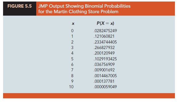
Statistical software packages also provide a capability for computing binomial probab­ilities. Consider the Martin Clothing Store example with n = 10 and p = .30. Figure 5.5 shows the binomial probabilities generated by JMP for all possible values of x. Note that these values are the same as those found in the p = .30 column of Table 5.14. The chapter appendices contain step-by-step instructions for using widely available software packages to generate binomial probabilities.

4. Expected Value and Variance for the Binomial Distribution

In Section 5.3 we provided formulas for computing the expected value and variance of a discrete random variable. In the special case where the random variable has a bi­nomial distribution with a known number of trials n and a known probability of success p, the general formulas for the expected value and variance can be simplified. The results follow.

For the Martin Clothing Store problem with three customers, we can use equation (5.13) to compute the expected number of customers who will make a purchase.

E(x) = np = 3(.30) = .9

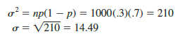
Suppose that for the next month the Martin Clothing Store forecasts 1000 customers will enter the store. What is the expected number of customers who will make a pur­chase? The answer is m = np = (1000)(.3) = 300. Thus, to increase the expected number of purchases, Martin’s must induce more customers to enter the store and/or somehow increase the probability that any individual customer will make a purchase after entering.

For the Martin Clothing Store problem with three customers, we see that the variance and standard deviation for the number of customers who will make a purchase are

For the next 1000 customers entering the store, the variance and standard deviation for the number of customers who will make a purchase are

Source:  Anderson David R., Sweeney Dennis J., Williams Thomas A. (2019), Statistics for Business & Economics, Cengage Learning; 14th edition.