Population Mean: σ Known

In Chapter 8 we said that the σ known case corresponds to applications in which historical data and/or other information are available that enable us to obtain a good estimate of the population standard deviation prior to sampling. In such cases the population standard de­viation can, for all practical purposes, be considered known. In this section we show how to conduct a hypothesis test about a population mean for the σ known case.

The methods presented in this section are exact if the sample is selected from a popula­tion that is normally distributed. In cases where it is not reasonable to assume the popu­lation is normally distributed, these methods are still applicable if the sample size is large enough. We provide some practical advice concerning the population distribution and the sample size at the end of this section.

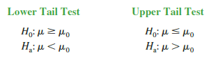
1. One-Tailed Test

One-tailed tests about a population mean take one of the following two forms.

Let us consider an example involving a lower tail test.

The Federal Trade Commission (FTC) periodically conducts statistical studies designed to test the claims that manufacturers make about their products. For example, the label on a large can of Hilltop Coffee states that the can contains 3 pounds of coffee. The FTC knows that Hilltop’s production process cannot place exactly 3 pounds of coffee in each can, even if the mean filling weight for the population of all cans filled is 3 pounds per can. However, as long as the population mean filling weight is at least 3 pounds per can, the rights of consumers will be protected. Thus, the FTC interprets the label information on a large can of coffee as a claim by Hilltop that the population mean filling weight is at least 3 pounds per can. We will show how the FTC can check Hilltop’s claim by conducting a lower tail hypothesis test.

The first step is to develop the null and alternative hypotheses for the test. If the population mean filling weight is at least 3 pounds per can, Hilltop’s claim is correct. This establishes the null hypothesis for the test. However, if the population mean weight is less than 3 pounds per can, Hilltop’s claim is incorrect. This establishes the alternative hypothesis. With m denoting the population mean filling weight, the null and alternative hypotheses are as follows:

Note that the hypothesized value of the population mean is μ₀ = 3.

If the sample data indicate that H₀ cannot be rejected, the statistical evidence does not support the conclusion that a label violation has occurred. Hence, no action should be taken against Hilltop. However, if the sample data indicate H₀ can be rejected, we will conclude that the alternative hypothesis, H_a: μ < 3, is true. In this case a conclusion of underfilling and a charge of a label violation against Hilltop would be justified.

Suppose a sample of 36 cans of coffee is selected and the sample mean X is computed as an estimate of the population mean μ. If the value of the sample mean X is less than 3 pounds, the sample results will cast doubt on the null hypothesis. What we want to know is how much less than 3 pounds must X be before we would be willing to declare the difference significant and risk making a Type I error by falsely accusing Hilltop of a label violation. A key factor in addressing this issue is the value the decision maker selects for the level of significance.

As noted in the preceding section, the level of significance, denoted by a, is the probability of making a Type I error by rejecting H₀ when the null hypothesis is true as an equality. The decision maker must specify the level of significance. If the cost of making a Type I error is high, a small value should be chosen for the level of significance. If the cost is not high, a larger value is more appropriate. In the Hilltop Coffee study, the director of the FTC’s testing program made the following statement: “If the company is meeting its weight specifications at μ = 3, I do not want to take action against them. But, I am willing to risk a 1% chance of making such an error.” From the director’s statement, we set the level of significance for the hypothesis test at a = .01. Thus, we must design the hypo­thesis test so that the probability of making a Type I error when μ = 3 is .01.

For the Hilltop Coffee study, by developing the null and alternative hypotheses and specifying the level of significance for the test, we carry out the first two steps required in conducting every hypothesis test. We are now ready to perform the third step of hypothesis testing: collect the sample data and compute the value of what is called a test statistic.

Test statistic For the Hilltop Coffee study, previous FTC tests show that the population standard deviation can be assumed known with a value of σ = .18. In addition, these tests also show that the population of filling weights can be assumed to have a normal distri­bution. From the study of sampling distributions in Chapter 7 we know that if the popu­lation from which we are sampling is normally distributed, the sampling distribution of X will also be normally distributed. Thus, for the Hilltop Coffee study, the sampling distri­bution of X is normally distributed. With a known value of σ = .18 and a sample size of n = 36, Figure 9.1 shows the sampling distribution of X when the null hypothesis is true as an equality; that is, when μ = μ₀ = 3.^[1] Note that the standard error of X is given by σ_X = σ/√n = .18/√36 = .03.

Because the sampling distribution of X is normally distributed, the sampling distribution of is a standard normal distribution. A value of z = -1 means that the value of X is one stand­ard error below the hypothesized value of the mean, a value of z = -2 means that the value of X is two standard errors below the hypothesized value of the mean, and so on. We can use the standard normal probability table to find the lower tail probability corresponding to any z value. For instance, the lower tail area at z = -3.00 is .0013. Hence, the probability of obtaining a value of z that is three or more standard errors below the mean is .0013. As a result, the probability of obtaining a value of X that is 3 or more standard errors below the hypothesized population mean m₀ = 3 is also .0013. Such a result is unlikely if the null hypothesis is true.

For hypothesis tests about a population mean in the σ known case, we use the stand­ard normal random variable z as a test statistic to determine whether X deviates from the hypothesized value of μ enough to justify rejecting the null hypothesis. With σ_X = σ/√n, the test statistic is as follows.

The key question for a lower tail test is, How small must the test statistic z be before we choose to reject the null hypothesis? Two approaches can be used to answer this question: the p-value approach and the critical value approach.

p-value approach The p-value approach uses the value of the test statistic z to compute a probability called a p-value.

The p-value is used to determine whether the null hypothesis should be rejected.

Let us see how the p-value is computed and used. The value of the test statistic is used to compute the p-value. The method used depends on whether the test is a lower tail, an upper tail, or a two-tailed test. For a lower tail test, the p-value is the probability of obtaining a value for the test statistic as small as or smaller than that provided by the sample. Thus, to compute the p-value for the lower tail test in the s known case, we use the standard normal distribution to find the probability that z is less than or equal to the value of the test statistic. After computing the p-value, we must then decide whether it is small enough to reject the null hypothesis; as we will show, this decision involves comparing the p-value to the level of significance.

Let us now compute the p-value for the Hilltop Coffee lower tail test. Suppose the sample of 36 Hilltop coffee cans provides a sample mean of X = 2.92 pounds. Is X = 2.92 small enough to cause us to reject H₀? Because this is a lower tail test, the p-value is the area under the standard normal curve for values of z < the value of the test statistic. Using X = 2.92, σ = .18, and n = 36, we compute the value of the test statistic z.

Thus, the p-value is the probability that z is less than or equal to -2.67 (the lower tail area corresponding to the value of the test statistic).

Using the standard normal probability table, we find that the lower tail area at z = -2.67 is .0038. Figure 9.2 shows that X = 2.92 corresponds to z = -2.67 and a p-value = .0038. This p-value indicates a small probability of obtaining a sample mean of X = 2.92 (and a test statistic of -2.67) or smaller when sampling from a population with μ = 3. This p-value does not provide much support for the null hypothesis, but is it small enough to cause us to reject H₀? The answer depends upon the level of significance for the test.

As noted previously, the director of the FTC’s testing program selected a value of .01 for the level of significance. The selection of a = .01 means that the director is willing to tolerate a probability of .01 of rejecting the null hypothesis when it is true as an equality (m₀ = 3). The sample of 36 coffee cans in the Hilltop Coffee study resulted in a p-value = .0038, which means that the probability of obtaining a value of X = 2.92 or less when the null hypothesis is true as an equality is .0038. Because .0038 is less than or equal to a = .01, we reject H₀. Therefore, we find sufficient statistical evidence to reject the null hypothesis at the .01 level of significance.

We can now state the general rule for determining whether the null hypothesis can be rejected when using the p-value approach. For a level of significance a, the rejection rule using the p-value approach is as follows:

In the Hilltop Coffee test, the p-value of .0038 resulted in the rejection of the null hypothesis. Although the basis for making the rejection decision involves a comparison of the p-value to the level of significance specified by the FTC director, the observed p-value of .0038 means that we would reject H₀ for any value of a > .0038. For this reason, the p-value is also called the observed level of significance.

Different decision makers may express different opinions concerning the cost of making a Type I error and may choose a different level of significance. By providing the p-value as part of the hypothesis testing results, another decision maker can compare the reported p-value to his or her own level of significance and possibly make a different decision with respect to rejecting H₀.

Critical value approach The critical value approach requires that we first determine a value for the test statistic called the critical value. For a lower tail test, the critical value serves as a benchmark for determining whether the value of the test statistic is small enough to reject the null hypothesis. It is the value of the test statistic that corresponds to an area of a (the level of significance) in the lower tail of the sampling distribution of the test statistic. In other words, the critical value is the largest value of the test statistic that will result in the rejection of the null hypothesis. Let us return to the Hilltop Coffee example and see how this approach works.

In the s known case, the sampling distribution for the test statistic z is a standard normal distribution. Therefore, the critical value is the value of the test statistic that corresponds to an area of a = .01 in the lower tail of a standard normal distribution. Using the standard normal probability table, we find that z = -2.33 provides an area of .01 in the lower tail (see Figure 9.3). Thus, if the sample results in a value of the test statistic that is less than or equal to -2.33, the corresponding p-value will be less than or equal to .01; in this case, we should reject the null hypothesis. Hence, for the Hilltop Coffee study the critical value rejection rule for a level of significance of .01 is

In the Hilltop Coffee example, x = 2.92 and the test statistic is z = -2.67. Because z = -2.67 < -2.33, we can reject H₀ and conclude that Hilltop Coffee is underfilling cans.

We can generalize the rejection rule for the critical value approach to handle any level of significance. The rejection rule for a lower tail test follows.

Summary The p-value approach to hypothesis testing and the critical value approach will always lead to the same rejection decision; that is, whenever the p-value is less than or equal to a, the value of the test statistic will be less than or equal to the critical value. The advantage of the p-value approach is that the p-value tells us how significant the results are (the observed level of significance). If we use the critical value approach, we only know that the results are significant at the stated level of significance.

At the beginning of this section, we said that one-tailed tests about a population mean take one of the following two forms:

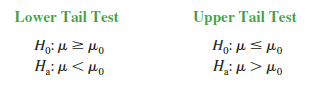
We used the Hilltop Coffee study to illustrate how to conduct a lower tail test. We can use the same general approach to conduct an upper tail test. The test statistic z is still computed using equation (9.1). But, for an upper tail test, the p-value is the probability of obtaining a value for the test statistic as large as or larger than that provided by the sample. Thus, to compute the p-value for the upper tail test in the s known case, we must use the standard normal distribution to find the probability that z is greater than or equal to the value of the test statistic. Using the critical value approach causes us to reject the null hypothesis if the value of the test statistic is greater than or equal to the critical value z_a; in other words, we reject H₀ if z ^ z_a.

Let us summarize the steps involved in computing p-values for one-tailed hypothesis tests.

COMPUTATION OF p-VALUES FOR ONE-TAILED TESTS

1. 1. Compute the value of the test statistic using equation (9.1).
   2. Lower tail test: Using the standard normal distribution, compute the prob­ability that z is less than or equal to the value of the test statistic (area in the lower tail).
   3. Upper tail test: Using the standard normal distribution, compute the prob­ability that z is greater than or equal to the value of the test statistic (area in the upper tail).

2. Two-Tailed Test

In hypothesis testing, the general form for a two-tailed test about a population mean is as follows:

H0: μ = μ0
Ha: μ # μ0

In this subsection we show how to conduct a two-tailed test about a population mean for the s known case. As an illustration, we consider the hypothesis testing situation facing MaxFlight, Inc.

The U.S. Golf Association (USGA) establishes rules that manufacturers of golf equip­ment must meet if their products are to be acceptable for use in USGA events. MaxFlight uses a high-technology manufacturing process to produce golf balls with a mean driv­ing distance of 295 yards. Sometimes, however, the process gets out of adjustment and produces golf balls with a mean driving distance different from 295 yards. When the mean distance falls below 295 yards, the company worries about losing sales because the golf balls do not provide as much distance as advertised. When the mean distance passes 295 yards, MaxFlight’s golf balls may be rejected by the USGA for exceeding the overall distance standard concerning carry and roll.

MaxFlight’s quality control program involves taking periodic samples of 50 golf balls to monitor the manufacturing process. For each sample, a hypothesis test is conducted to determine whether the process has fallen out of adjustment. Let us develop the null and alternative hypotheses. We begin by assuming that the process is functioning correctly; that is, the golf balls being produced have a mean distance of 295 yards. This assumption establishes the null hypothesis. The alternative hypothesis is that the mean distance is not equal to 295 yards. With a hypothesized value of m₀ = 295, the null and alternative hypo­theses for the MaxFlight hypothesis test are as follows:

If the sample mean X is significantly less than 295 yards or significantly greater than 295 yards, we will reject H₀. In this case, corrective action will be taken to adjust the manu­facturing process. On the other hand, if X does not deviate from the hypothesized mean m₀ = 295 by a significant amount, H₀ will not be rejected and no action will be taken to adjust the manufacturing process.

The quality control team selected a = .05 as the level of significance for the test. Data from previous tests conducted when the process was known to be in adjustment show that the population standard deviation can be assumed known with a value of s = 12. Thus, with a sample size of n = 50, the standard error of X is

Because the sample size is large, the central limit theorem (see Chapter 7) allows us to conclude that the sampling distribution of X can be approximated by a normal distribution. Figure 9.4 shows the sampling distribution of X for the MaxFlight hypothesis test with a hypothesized population mean of m₀ = 295.

Suppose that a sample of 50 golf balls is selected and that the sample mean is X = 297.6 yards. This sample mean provides support for the conclusion that the popu­lation mean is larger than 295 yards. Is this value of X enough larger than 295 to cause us to reject H₀ at the .05 level of significance? In the previous section we described two approaches that can be used to answer this question: the p-value approach and the critical value approach.

p-value approach Recall that the p-value is a probability used to determine whether the null hypothesis should be rejected. For a two-tailed test, values of the test statistic in either tail provide evidence against the null hypothesis. For a two-tailed test, the p-value is the probabil­ity of obtaining a value for the test statistic as unlikely as or more unlikely than that provided by the sample. Let us see how the p-value is computed for the MaxFlight hypothesis test.

First we compute the value of the test statistic. For the s known case, the test statistic z is a standard normal random variable. Using equation (9.1) with x = 297.6, the value of the test statistic is

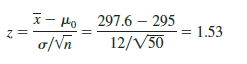
Now to compute the p-value we must find the probability of obtaining a value for the test statistic at least as unlikely as z = 1.53. Clearly values of z > 1.53 are at least as unlikely. But, because this is a two-tailed test, values of z < -1.53 are also at least as unlikely as the value of the test statistic provided by the sample. In Figure 9.5, we see that the two-tailed p-value in this case is given by P(z < -1.53) + P(z > 1.53). Because the normal curve is symmetric, we can compute this probability by finding the upper tail area at z = 1.53 and doubling it. The table for the standard normal distribution shows that P(z < 1.53) = .9370. Thus, the upper tail area is P(z > 1.53) = 1.0000 – .9370 = .0630. Doubling this, we find the p-value for the MaxFlight two-tailed hypothesis test is p-value = 2(.0630) = .1260.

Next we compare the p-value to the level of significance to see whether the null hy­pothesis should be rejected. With a level of significance of a = .05, we do not reject H₀ because the p-value = .1260 > .05. Because the null hypothesis is not rejected, no action will be taken to adjust the MaxFlight manufacturing process.

The computation of the p-value for a two-tailed test may seem a bit confusing as com­pared to the computation of the p-value for a one-tailed test. But it can be simplified by following three steps.

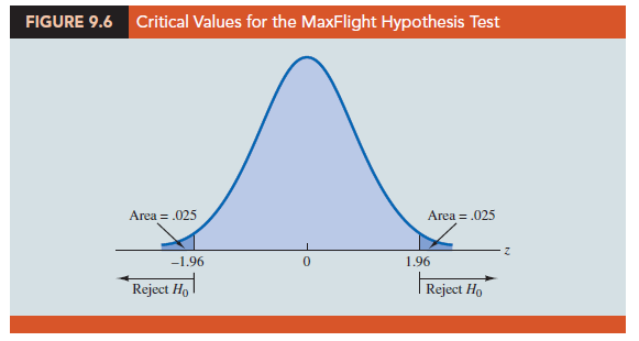
Critical value approach Before leaving this section, let us see how the test statistic z can be compared to a critical value to make the hypothesis testing decision for a two-tailed test. Figure 9.6 shows that the critical values for the test will occur in both the lower and upper tails of the standard normal distribution. With a level of significance of a = .05, the area in each tail corresponding to the critical values is a/2 = .05/2 = .025. Using the standard normal probability table, we find the critical values for the test statistic are -z.₀₂₅ = -1 96 and z.₀₂₅ = 1.96. Thus, using the critical value approach, the two-tailed rejection rule is

Because the value of the test statistic for the MaxFlight study is z = 1.53, the statistical evidence will not permit us to reject the null hypothesis at the .05 level of significance.

3. Summary and Practical Advice

We presented examples of a lower tail test and a two-tailed test about a population mean. Based upon these examples, we can now summarize the hypothesis testing procedures about a population mean for the s known case as shown in Table 9.2. Note that m₀ is the hypothesized value of the population mean.

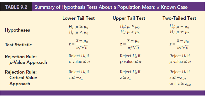
The hypothesis testing steps followed in the two examples presented in this section are common to every hypothesis test.

Practical advice about the sample size for hypothesis tests is similar to the advice we provided about the sample size for interval estimation in Chapter 8. In most applications, a sample size of n > 30 is adequate when using the hypothesis testing procedure described in this section. In cases where the sample size is less than 30, the distribution of the popula­tion from which we are sampling becomes an important consideration. If the population is normally distributed, the hypothesis testing procedure that we described is exact and can be used for any sample size. If the population is not normally distributed but is at least roughly symmetric, sample sizes as small as 15 can be expected to provide acceptable results.

4. Relationship Between Interval Estimation and Hypothesis Testing

In Chapter 8 we showed how to develop a confidence interval estimate of a population mean. For the s known case, the (1 – a)% confidence interval estimate of a population mean is given by

In this chapter, we showed that a two-tailed hypothesis test about a population mean takes the following form:

where m₀ is the hypothesized value for the population mean.

Suppose that we follow the procedure described in Chapter 8 for constructing a 100(1 – a)% confidence interval for the population mean.We know that 100(1 – a)% of the confidence intervals generated will contain the population mean and 100a% of the confidence intervals generated will not contain the population mean. Thus, if we reject H₀ whenever the confidence interval does not contain m₀, we will be rejecting the null hypothesis when it is true (μ = μ₀) with probability a. Recall that the level of significance is the prob­ability of rejecting the null hypothesis when it is true. So constructing a 100(1 – a)% con­fidence interval and rejecting H₀ whenever the interval does not contain m₀ is equivalent to conducting a two-tailed hypothesis test with a as the level of significance. The procedure for using a confidence interval to conduct a two-tailed hypothesis test can now be summarized.

Let us illustrate by conducting the MaxFlight hypothesis test using the confidence inter­val approach. The MaxFlight hypothesis test takes the following form:

To test these hypotheses with a level of significance of a = .05, we sampled 50 golf balls and found a sample mean distance of X = 297.6 yards. Recall that the population standard deviation is s = 12. Using these results with z.₀₂₅ = 1.96, we find that the 95% confidence interval estimate of the population mean is

This finding enables the quality control manager to conclude with 95% confidence that the mean distance for the population of golf balls is between 294.3 and 300.9 yards. Because the hypothesized value for the population mean, m₀ = 295, is in this interval, the hypothesis testing conclusion is that the null hypothesis, H₀: m = 295, cannot be rejected.

Note that this discussion and example pertain to two-tailed hypothesis tests about a population mean. However, the same confidence interval and two-tailed hypothesis testing relationship exists for other population parameters. The relationship can also be extended to one-tailed tests about population parameters. Doing so, however, requires the develop­ment of one-sided confidence intervals, which are rarely used in practice.

Source:  Anderson David R., Sweeney Dennis J., Williams Thomas A. (2019), Statistics for Business & Economics, Cengage Learning; 14th edition.