In this section we describe how to conduct hypothesis tests about a population mean for the σ unknown case. Because the σ unknown case corresponds to situations in which an estimate of the population standard deviation cannot be developed prior to sampling, the sample must be used to develop an estimate of both μ and σ. Thus, to conduct a hypothesis test about a population mean for the s unknown case, the sample mean X is used as an estimate of m and the sample standard deviation 5 is used as an estimate of σ.
The steps of the hypothesis testing procedure for the σ unknown case are the same as those for the s known case described in Section 9.3. But, with s unknown, the computation of the test statistic and p-value is a bit different. Recall that for the s known case, the sampling distribution of the test statistic has a standard normal distribution. For the σ unknown case, however, the sampling distribution of the test statistic follows the t distribution; it has slightly more variability because the sample is used to develop estimates of both m and σ.
In Section 8.2 we showed that an interval estimate of a population mean for the σ unknown case is based on a probability distribution known as the t distribution. Hypothesis tests about a population mean for the σ unknown case are also based on the t distribution. For the σ unknown case, the test statistic has a t distribution with n – 1 degrees of freedom.

In Chapter 8 we said that the t distribution is based on an assumption that the population from which we are sampling has a normal distribution. However, research shows that this assumption can be relaxed considerably when the sample size is large enough. We provide some practical advice concerning the population distribution and sample size at the end of the section.
1. One-Tailed Test
Let us consider an example of a one-tailed test about a population mean for the s unknown case. A business travel magazine wants to classify transatlantic gateway airports according to the mean rating for the population of business travelers. A rating scale with a low score of 0 and a high score of 10 will be used, and airports with a population mean rating greater than 7 will be designated as superior service airports. The magazine staff surveyed a sample of 60 business travelers at each airport to obtain the ratings data. The sample for London’s Heathrow Airport provided a sample mean rating of X = 7.25 and a sample standard deviation of s = 1.052. Do the data indicate that Heathrow should be designated as a superior service airport?
We want to develop a hypothesis test for which the decision to reject H0 will lead to the conclusion that the population mean rating for the Heathrow Airport is greater than 7. Thus, an upper tail test with Ha: μ > 7 is required. The null and alternative hypotheses for this upper tail test are as follows:

We will use a = .05 as the level of significance for the test.
Using equation (9.2) with X = 7.25, μ0 = 7, 5 = 1.052, and n = 60, the value of the test statistic is

The sampling distribution of t has n – 1 = 60 – 1 = 59 degrees of freedom. Because the test is an upper tail test, the p-value is P (t > 1.84), that is, the upper tail area corresponding to the value of the test statistic.
The t distribution table provided in most textbooks will not contain sufficient detail to determine the exact p-value, such as the p-value corresponding to t = 1.84. For instance, using Table 2 in Appendix B, the t distribution with 59 degrees of freedom provides the following information.

We see that t = 1.84 is between 1.671 and 2.001. Although the table does not provide the exact p-value, the values in the “Area in Upper Tail” row show that the p-value must be less than .05 and greater than .025. With a level of significance of a = .05, this placement is all we need to know to make the decision to reject the null hypothesis and conclude that Heathrow should be classified as a superior service airport.
Because it is cumbersome to use a t table to compute p-values, and only approximate values are obtained, we show how to compute the exact p-value using Excel or JMP. Using Excel or JMP with t = 1.84 provides the upper tail p-value of .0354 for the Heathrow Airport hypothesis test. With .0354 < .05, we reject the null hypothesis and conclude that Heathrow should be classified as a superior service airport.
The decision whether to reject the null hypothesis in the s unknown case can also be made using the critical value approach. The critical value corresponding to an area of a = .05 in the upper tail of a t distribution with 59 degrees of freedom is t05 = 1.671. Thus the rejection rule using the critical value approach is to reject H0 if t > 1.671. Because t = 1.84 > 1.671, H0 is rejected. Heathrow should be classified as a superior service airport.
2. Two-Tailed Test
To illustrate how to conduct a two-tailed test about a population mean for the s unknown case, let us consider the hypothesis testing situation facing Holiday Toys. The company manufactures and distributes its products through more than 1000 retail outlets. In planning production levels for the coming winter season, Holiday must decide how many units of each product to produce prior to knowing the actual demand at the retail level.
For this year’s most important new toy, Holiday’s marketing director is expecting demand to average 40 units per retail outlet. Prior to making the final production decision based upon this estimate, Holiday decided to survey a sample of 25 retailers in order to develop more information about the demand for the new product. Each retailer was provided with information about the features of the new toy along with the cost and the suggested selling price. Then each retailer was asked to specify an anticipated order quantity.
With μ denoting the population mean order quantity per retail outlet, the sample data will be used to conduct the following two-tailed hypothesis test:

If H0 cannot be rejected, Holiday will continue its production planning based on the marketing director’s estimate that the population mean order quantity per retail outlet will be μ = 40 units. However, if H0 is rejected, Holiday will immediately reevaluate its production plan for the product. A two-tailed hypothesis test is used because Holiday wants to reevaluate the production plan if the population mean quantity per retail outlet is less than anticipated or greater than anticipated. Because no historical data are available (it’s a new product), the population mean m and the population standard deviation must both be estimated using X and 5 from the sample data.
The sample of 25 retailers provided a mean of X = 37.4 and a standard deviation of 5 = 11.79 units. Before going ahead with the use of the t distribution, the analyst constructed a histogram of the sample data in order to check on the form of the population distribution. The histogram of the sample data showed no evidence of skewness or any extreme outliers, so the analyst concluded that the use of the t distribution with n – 1 = 24 degrees of freedom was appropriate. Using equation (9.2) with X = 37.4, μ0 = 40, 5 = 11.79, and n = 25, the value of the test statistic is

Because we have a two-tailed test, the p-value is two times the area under the curve of the t distribution for t < -1.10. Using Table 2 in Appendix B, the t distribution table for 24 degrees of freedom provides the following information.

The t distribution table only contains positive t values. Because the t distribution is symmetric, however, the upper tail area at t = 1.10 is the same as the lower tail area at t = -1.10. We see that t = 1.10 is between .857 and 1.318. From the “Area in Upper Tail” row, we see that the area in the upper tail at t = 1.10 is between .20 and .10.
When we double these amounts, we see that the p-value must be between .40 and .20. With a level of significance of a = .05, we now know that the p-value is greater than a. Therefore, H0 cannot be rejected. Sufficient evidence is not available to conclude that Holiday should change its production plan for the coming season.
Appendix F shows how the p-value for this test can be computed using Excel or JMP. The p-value obtained is .2822. With a level of significance of a = .05, we cannot reject H0 because .2822 > .05.
The test statistic can also be compared to the critical value to make the two-tailed hypothesis testing decision. With a = .05 and the t distribution with 24 degrees of freedom, —t.025 = -2.064 and t.025 = 2.064 are the critical values for the two-tailed test. The rejection rule using the test statistic is
![]()
Based on the test statistic t = -1.10, H0 cannot be rejected. This result indicates that Holiday should continue its production planning for the coming season based on the expectation that m = 40.
3. Summary and Practical Advice
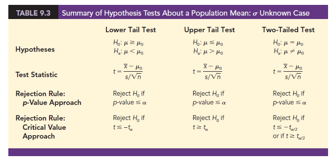
Table 9.3 provides a summary of the hypothesis testing procedures about a population mean for the s unknown case. The key difference between these procedures and the ones for the s known case is that 5 is used, instead of s, in the computation of the test statistic. For this reason, the test statistic follows the t distribution.
The applicability of the hypothesis testing procedures of this section is dependent on the distribution of the population being sampled from and the sample size. When the population is normally distributed, the hypothesis tests described in this section provide exact results for any sample size. When the population is not normally distributed, the procedures are approximations. Nonetheless, we find that sample sizes of 30 or greater will provide good results in most cases. If the population is approximately normal, small sample sizes (e.g., n < 15) can provide acceptable results. If the population is highly skewed or contains outliers, sample sizes approaching 50 are recommended.
Source: Anderson David R., Sweeney Dennis J., Williams Thomas A. (2019), Statistics for Business & Economics, Cengage Learning; 14th edition.
28 Aug 2021
28 Aug 2021
28 Aug 2021
30 Aug 2021
31 Aug 2021
30 Aug 2021