Repeated-Measures and Mixed ANOVAs with SPSS: The Product Data Set

• Open the SPSS for Windows program. Open the Product data set. Do not retrieve the hsbdataNew for this assignment.

In this study, each of the 12 participants (or subjects) has evaluated four products that vary in cost (e.g., four brands of DVD players) on 1-7 Likert scales. Product A is the most expensive (i.e., $400), Product B is less expensive (i.e., $300), Product C costs only $200, and Product D is $100. You will find the data presented in the SPSS data editor once you have opened the product data set.

• Click on the Data View tab at the bottom of the screen to get Fig 10.1.

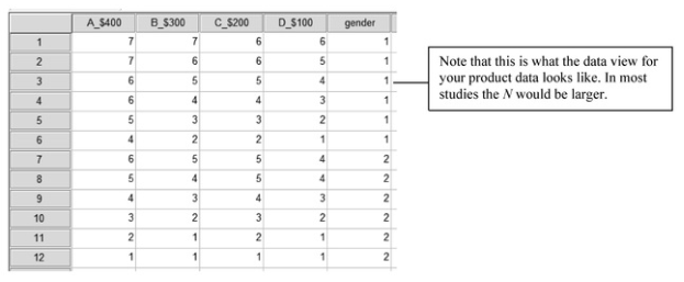
Fig. 10.1. Data view for the product data.

Figure 10.1 shows the Data View for 12 participants who were asked to rate four products (A_$400,B_$300, C_$200, D_$100) from 1 (very low quality) to 7 (very high quality). The participants were also asked their gender (1 = male, 2 = female). Thus, subjects 1-6 are males, and 7-12 are females.

• Click on the Variable View tab to see the names and labels of the variables as shown in Fig. 10.2.

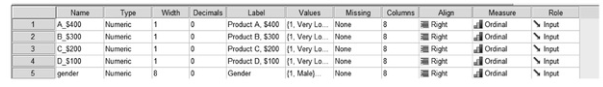
Fig. 10.2. Variable view.

We have labeled the measurement of the four products scale because the frequency distribution of each is approximately normal. We label gender and other dichotomous variables as nominal; however, despite this traditional designation for dichotomous variables, dichotomous variables, unlike other types of nominal variables, provide meaningful averages (indicating percentage of participants falling in each category) and can be used in multiple and logistic regression as if they were ordered. Furthermore, many dichotomous variables (but not gender) even have an implied order (e.g., 0 = do not have the characteristic and 1 = have the characteristic; thus, a score of 1 indicates more of the characteristic than does a score of 0).

In repeated-measures (also called within-subjects) analyses, SPSS creates the Within-Subjects Factor or independent variable from two or more existing variables (in this case A_$400, B_$300, C_$200, D_$100). These then become levels of the new independent variable. In this example, we will call the new variable product, and it has four levels (A_$400, etc.), indicating which product was being rated. In order for a set of variables to be converted into a meaningful within-subject factor, the scores on each of the existing variables (which will become levels of the new within-subjects variable) have to be comparable (e.g., ratings on the same seven-point Likert scale) and each participant has to have a score on each of the variables. The within-subject factor could be based on related or matched subjects (e.g., the ratings of a product by mother, father, and child from each family) instead of a single participant having repeated scores. The within-subjects design should be used whenever there are known dependencies in the data, such as when the same questions are systematically asked of multiple family members (e.g., there is a mother, father, and child rating for each family) that would otherwise violate the between-subjects assumption of independent observations. The dependent variable for the data in Fig. 10.1 could be called product ratings and would be the scores/ratings for each of the four products. Thus, the independent variable, product, indicates which product is being rated, and the dependent variable is the rating itself. Note that gender is a between-subjects independent variable that will be used in Problem 10.3.

Source: Leech Nancy L. (2014), IBM SPSS for Intermediate Statistics, Routledge; 5th edition;

download Datasets and Materials.