What could you do if the product ratings are ordinal data or the repeated- measures ANOVA assumptions are markedly violated? One answer is to use a nonparametric statistic. As you can tell from Table 5.1, an appropriate nonparametric test for when you have more than two levels of one repeated- measures or related samples (i.e., within-subjects) independent variables is the Friedman test.
10.2 Are there differences among the mean ranks of the product ratings?
Let’s use A_$400 to D_$100 again with the following commands:
- Analyze → Nonparametric tests →Legacy Dialogs→ K Related Samples… and move product A [A_$400] to product D [D_$100] to the Test Variables box (see 10.7).
- Make sure the Friedman test type is checked.
- Then click on Statistics to get 10.8.
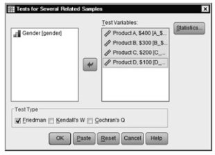
Fig. 10.7. Tests for several related samples.
- Now click on Descriptive.
- Click on Continue, then OK. Look at your output and compare it to Output 10.2a.
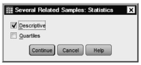
Fig. 10.8. Descriptive statistics for nonparametric tests for several related samples.
Output 10.2a: Nonparametric Tests With Four Related Samples
NPAR TESTS
/STATISTICS DESCRIPTIVES /MISSING LISTWISE.
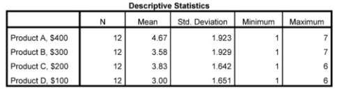

Interpretation of Output 10.2a
The Descriptive Statistics table provides familiar statistics that were useful for interpreting the polynomial contrasts in Output 10.1 but are not themselves used in the Friedman test. Rather, ratings are ranked, and the means of these ranks are used in the Friedman test. The Ranks table shows the mean rank for each of the four products.
There is not an easy method for calculating effect sizes for the Friedman test. Therefore, we recommend focusing on calculating effect sizes for any follow-up tests that you might do. Below, we will show you how to calculate an effect size for the follow-up Wilcoxon test.
The Friedman Test Statistics table shows the results of the null hypothesis that the four related variables come from the same population. For each rater/case, the four variables are ranked from 1 to 4, with 4 being the highest rank. The test statistic is based on these ranks. The Asymp. Sig. (asymptotic significance) means this is not an exact significance level. The p <.001 indicates that there is a statistically significant overall difference among the four mean ranks.
In order to determine which pairs of differences between mean ranks are significant, and thus the likely source of the significant Friedman test, we will perform a nonparametric related-sample test, the Wilcoxon. See Table 5.1 for a more complete view of the different statistical tests used to compare samples.
- Analyze → Nonparametric tests → Legacy Dialogs → 2 Related Samples and make sure that Wilcoxon is checked.
- Then highlight both Product A, $400 and Product B, $300 and click the arrow to move them over together.
- Next, repeat for Product B, $300 and Product C, $200 and for Product C, $200 and Product D, $100.
- Click OK.
Check to make sure that your syntax and output are like those in Output 10.2b.
Output 10.2b: Follow-Up Paired Comparisons for Significant
Friedman
NPAR TESTS
/WILCOXON=A_$400 B_$300 C_$200 WITH B_$300 C_$200 D_$100 (PAIRED) /MISSING ANALYSIS.
Wilcoxon Signed Ranks Test
a. Product B, $300 < Product A, $400
b. Product B, $300 > Product A, $400
c. Product B, $300 = Product A, $400
d. Product C, $200 < Product B, $300
e. Product C, $200 > Product B, $300
f. Product C, $200 = Product B, $300
g. Product D, $100 < Product C, $200
h. Product D, $100 > Product C, $200
i. Product D, $100 = Product C, $200
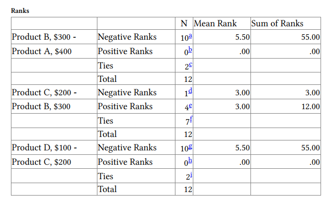
Interpretation of Output 10.2b
Given that there was a significant overall difference between the mean ranks, we followed up the Friedman with Wilcoxon tests. Since the products are ordered and there are four levels, it makes sense to do three orthogonal contrasts, contrasting adjacent pairs. A larger number of comparisons would prevent the comparisons from being independent of one another. Given that three post hoc comparisons were made, it would be desirable to make a Bonferroni correction on alpha, such that p would need to be .05/3 (.017) to be significant. Notice that the contrasts between products 2 and 1 and between 4 and 3 are significant at this level and that they both indicate that the higher numbered product was given a lower rating than the lower numbered product. On the other hand, the difference between ratings for products 3 and 2 was not significant. This is not surprising when you look at the mean ranks in Output 10.2a and suggests that the slight increase in ratings for Product C compared to Product B may not be important. Remember, however, that the Wilcoxon is not performed on the rating scores themselves but rather on the ranks of the ratings.
To calculate an effect size for this analysis, we can compute an r from the z scores and Ns (Total) that are shown in Output 10.2b using the formula
vW For Output 10.2b, r = -.84 (i.e., -2.919/3.46) for the comparison of Product A with Product B. For the comparison of Product C with Product D, r = -.91 (i.e., -3.162/3.46). Both of these are very large effect sizes.
Example of How to Write About Outputs 10.2a and 10.2b
Results
A Friedman test was conducted to assess if there were differences among the mean ranks of the product ratings. (Assumptions of independence of observations and continuous distributions were checked and met.) A statistically significant difference was found, x2 (3, N = 12) = 26.17, p = .001. This indicates that there were differences among the four mean ranks. Three orthogonal contrasts were performed using Wilcoxon tests with the Bonferroni correction (comparison-wise alpha = .017). The contrasts between Products 1 and 2 (Z = -2.92, p = .004, r = -.84), and between Products 3 and 4 (Z = -3.16, p = .002, r = -.91) were found to be statistically significant; however that between Products 2 and 3 was not statistically significant. In both cases, the statistically significant contrasts indicated that the more expensive product was rated more highly, and the differences were very large according to Cohen (1988).
Source: Leech Nancy L. (2014), IBM SPSS for Intermediate Statistics, Routledge; 5th edition;
download Datasets and Materials.
30 Mar 2023
14 Sep 2022
22 Sep 2022
29 Mar 2023
29 Mar 2023
27 Mar 2023