Problem 12.1: Unconditional Level 1 Repeated-Measures Model with SPSS

Although one can use GLM to compute analyses of repeated-measures data, as shown in Chapter 10, multilevel models often are more useful for analyzing repeated-measures data for several reasons. First, it is possible to use multilevel models even if there is some incomplete information on some participants or if their data are from different time points (see Chapter 13). Second, one can model differently shaped growth curves more readily in multilevel models. Finally, one can select the best variance-covariance structure for the data and specify only the interactions of interest for the analyses. In a repeated-measures design, the Level 1 model describes the repeated measures data for the participants and Level 2 involves variables that measure systematic differences among the participants, in which the repeated measures are nested, that might help explain the pattern of change in the repeated measures. Typically, the first step in undertaking multilevel linear modeling is to determine whether there is sufficient variability at Level 1 to require explanation by Level 2 variables. The unconditional Level 1 model answers this question:

12.1 Is there significant variability among participants in the average Distance (in mm from center of pituitary to pteryomaxillary fissure) across ages? Is there a linear relation between the withinsubject variable, Age, and Distance? Is there a quadratic relation between Age and Distance?

Before we do the analysis to answer these questions, we will calculate descriptive statistics and do a boxplot to help us in answering them.

• First, compute descriptive statistics by clicking on Analyze → Descriptive Statistics → Explore.
• Click on Distance and move it into Dependent List: box (see 12.1).
• Click on Age and move it into the Factor List: box.
• Check to be sure Both is selected under Display.

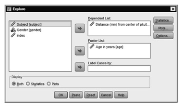
Fig. 12.1. Explore.

• Click on OK.
• Compare your output and syntax with Output 12.1a.

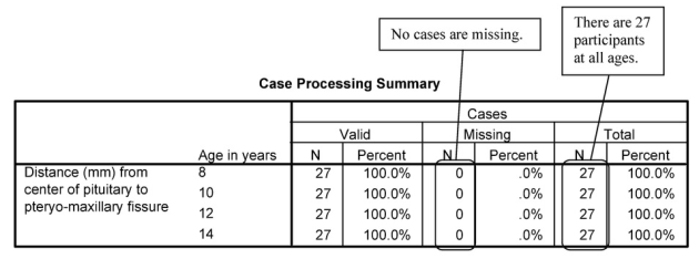
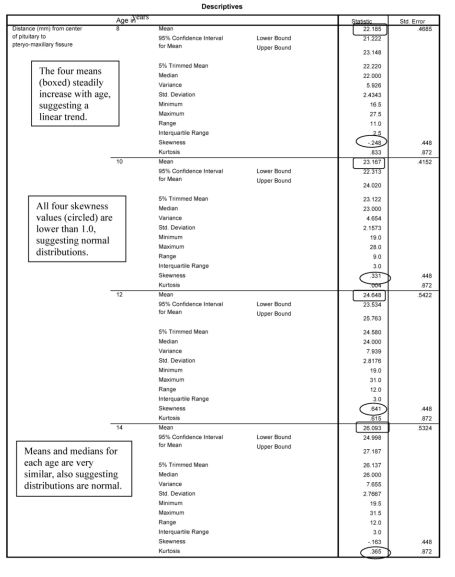
Output 12.1a: Descriptive Statistics for Distance as a Function of Age

EXAMINE VARIABLES=distance BY age /PLOT BOXPLOT STEMLEAF /COMPARE GROUPS

/STATISTICS DESCRIPTIVES

/CINTERVAL 95

/MISSING LISTWISE

/NOTOTAL.

Explore Age in years

Interpretation of Output 12.1a

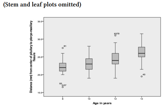
First, we examine the output from the Explore program, which provides us with descriptive statistics for the distance variable at each age period. We have omitted the stem-and-leaf plots to conserve space because we can obtain the most pertinent information from the tables and boxplot.

The first table in Output 12.1a shows us that there were 27 children at each age, so there was no attrition over time, and none were missing data on distance at any age. The Descriptives table shows that at age 8, the average distance (mm from the center of the pituitary to the pteryomaxillary fissure) was 22.19 (SD = 2.43); at 10, 12, and 14, the mean distances were 23.17, 24.65, and 26.09, respectively, with corresponding standard deviations of 2.16, 2.82, and 2.77. These numbers, along with the boxplots, suggest that distance increases in a linear manner; however, to see if there is one change in direction/rate of change (and to show you how to do polynomial trends), we will also look at a quadratic trend for age.

Now we will answer our research questions: Is there significant variability among participants in the average Distance (in mm from center of pituitary to pteryomaxillary fissure) across ages? Is there a linear relation between Age and Distance? Is there a quadratic relation between Age and Distance?

• Select Analyze → Mixed Models → Linear.
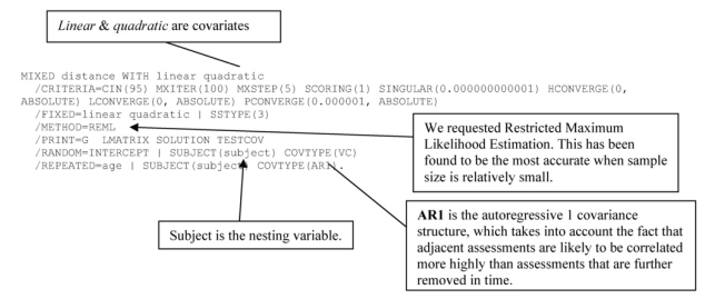
• Highlight Subject and move it to the Subjects: box (see 12.2 for help). Note that Subjects is a way to specify the lowest independent level of data (the level in which the lowest level of data is nested). In this case, it involves the Subject variable, because observations are nested in subjects.
• Highlight Age (Age in years) and move it into the Repeated: box, specifying the repeated-measures variable. This models withinsubject variance, as distinguished from the between-subject variance modeled by the Random
• Click on the arrow next to Repeated covariance type, and change Diagonal to specify AR(1), as shown in 12.2. This is an autoregressive covariance structure with homogeneous variances, with a lag of 1 (one age level in this case). The autoregressive structure indicates that each person’s distance measurement at one time is correlated with his or her distance measurement at the previous time period, which is typical of a repeated-measures situation.

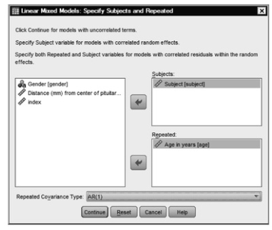
Fig. 12.2. Linear mixed models: Specify subjects and repeated.

• Click on Continue. This will open the Linear Mixed Models window (Fig- 12.3).
• Click on Distance and move it into the Dependent Variable: box.
• Click on Linear and move it into the Covariate(s): box.
• Click on Quadratic and move it into the Covariate(s): box. We have created these two variables to look at the linear and quadratic effects of age, referenced to the youngest age. Note that these really get at the effects of age, even though they are separate variables, because they correspond to the different levels of Age in the dataset. Both consist of weights beginning with 0, which causes SPSS to use the initial age level as the reference. The quadratic weights simply involve squaring the linear weights. So, linear weights are 0, 1, 2, 3 and quadratic are 0,1,4,9 (see Growth study.sav, linear and quadradic “variables”. We are not doing a cubic effect, so we will not use the cubic variable).

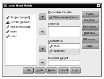
Fig. 12.3. Linear mixed models.

• Next, click on Fixed in the upper right-hand corner of 12.3 to get to Fig. 12.4.
• Click on the arrow next to Factorial and change Factorial to Main Effects.
• Click on linear and then on Add; this will move linear into the Model Repeat this for quadratic. Leave the defaults for the other options, making sure that Include intercept is checked and Type III sums of squares is in the box for sums of squares (see Fig. 12.4).

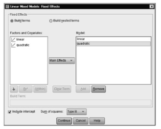
Fig. 12.4. Linear mixed models: Fixed effects.

• Click on Continue. This will take you back to 12.3.
• In the Linear Mixed Models window click on Random to get to 12.5.
• Under Random Effects check the box next to Include intercept. This will enable us to look at differences between the individual participants in mean score on the dependent variable.
• Leave the Covariance Type as Variance Components. In the Variance Component model, mean score across observations (intercept) is assumed to vary across individuals, but the slopes (predicting Distance from linear and quadratic curves in this case) are not expected to differ across individuals. Since all individuals are the same ages, this seems reasonable and keeps the model simpler.
• We have already included an autoregressive, repeated measures structure for the Age variable, and have entered fixed effects for the polynomial trend analysis, so we will not add any independent variables to the Random Effects.
• Under Subject Groupings, move Subject into the Combinations: box (see 12.5).

Fig. 12.5. Linear mixed models: Random effects.

• Click on Continue. This will take you back to 12.3.
• Click on Statistics. Select Parameter estimates, Test for covariance parameters, Covariances of random effects, and Contrast coefficient matrix (see 12.6).

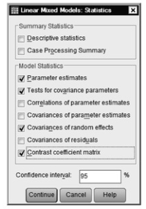
Fig. 12.6. Linear mixed models: Statistics.

• Click on Continue to go back to 12.3.
• Click on OK.
• Compare your output with Output 12.1b

Output 12.1b Unconditional Model for Age Nested in Subject

Interpretation of Output 12.1b

First, you see the log file, or syntax, indicating what you did. Note that you used REML (Restricted Maximum Likelihood) as your estimation method (the default method in SPSS, so we didn’t need to specify it). REML adjusts for the fixed effects, usually leading to a reduction in standard error. It has been found to be more accurate than Full Maximum Likelihood when there is a small number of entities (in this case, participants).

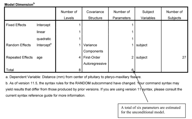
In the first table of Output 12.1b, Model Dimensions, we can check to make sure that everything is as we intended it and how many parameters are being estimated. We see that the intercept and Linear and Quadratic are fixed effects, age also is a repeated effect with a first-order autoregressive covariance structure, and Subject is a nesting variable. The repeated effects of age involve estimating two parameters: AR(1) rho, an estimate of the covariation between age periods and AR(1) diagonal, which is a measure of average within-age variance. Note that since linear and quadratic were
specified as covariates, they only have had one level listed, and dummy variables were not created.

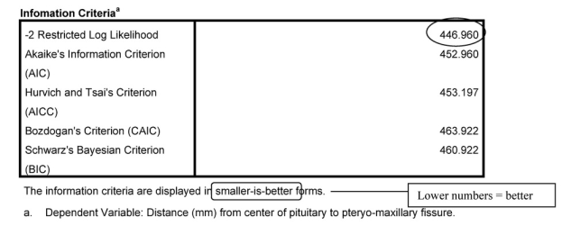
Next, we have information about the goodness of fit of the unconditional model. We can compare this to later models to see how much the goodness of fit is improved when predictors are added. Fit is better if the Information Criteria are smaller. The -2 restricted log likelihood criterion is a basic measure of goodness of fit of the model. The other four criteria are based on this same criterion, but they make adjustments for the complexity of the model.

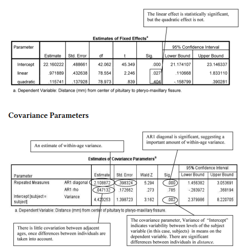
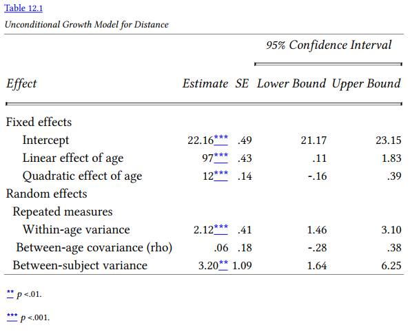
Interpretation of Output 12.1 continued In the Fixed Effects table, we see the intercept for the Distance variable (Intercept) and linear and quadratic effects of age. The t test for the intercept is testing whether the average Distance from the pituitary to the pteryomaxillary fissure, across individuals, is statistically significantly different from zero, which it is, t(42.06) = 45.35, p < .001; however, this is not really of interest. The t test for linear and quadratic are more familiar and more useful, testing whether the Distance variable changes statistically significantly in a linear and/or quadratic fashion across the four ages (8, 10, 12, and 14 years). We see that the linear growth curve is significant, t(78.55) = 2.25, p = .027. On the other hand, the quadratic growth curve is not significant, t(78.97) = .84, p =.40. We are omitting the Type III Estimable functions table from the output reproduced here to save space, but these show you how the computer program contrasted the dummy variables.

The Covariance Parameters table shows the variance estimates for the random and withinsubjects effects, along with a test of statistical significance. The AR(1) rho estimate is an intraclass correlation coefficient, indicating the extent to which the age periods are correlated. Adjacent age periods (e.g., 8 and 10 or 10 and 12) are correlated an average of rho; those separated by another age group (e.g., 8 and 12) are rho². In this case, rho is low (.047) and is not statistically significant. This means that rho² is estimated to be (.047)² or .0022 for the correlation between age groups that are separated by another group (8 and 12 or 10 and 14), suggesting quite negligible correlations between age groups that are further removed. These results suggest that, at least after taking into account effects of subjects, the contribution of autoregression is negligible. Under normal circumstances, we would modify our model of the random covariance based on this, but we will continue using AR1 in the next model so that we can show you how to compare a conditional model to an unconditional model with everything specified the same except for the new predictor. The AR1 diagonal estimate is the estimate of the variance within age periods, which in this case is high and significant, suggesting that there is significant variability within age that could be predicted by conditional model predictor(s). The final entry in this table (Intercept [subject = subject]) is for the variance component pertaining to variation between participants. It, too, is large and significant, suggesting that there is variability between subjects that could be explained using predictors in a conditional model. The statistical significance tests should be interpreted with caution, however; Wald Z test may be unreliable with small samples, such as those for this study.

Example of How to Write About Output 12.1

Results

The unconditional repeated-measures model revealed that there was significant variability in the distance measure, suggesting that it would be worthwhile to examine a conditional model that could potentially explain some of this variability. (The assumptions of independent observations at the level above the nesting, bivariate normality, linear relationships, and random residuals were checked and met.) The linear trend for age was a statistically significant predictor of changes in the distance measure, t(78.55) = 2.25, p = .027. On the other hand, the quadratic trend for age was not significant, indicating that age was related to the distance from center of pituitary to pteryomaxillary fissure measure in a linear manner. Examination of the means for the four age supported this, indicating that there was a steady, linear increase in the measure from age 8 until age 12 periods (M = 22.19, 23.17, 24.65, and 26.09; SD = 2.43, 2.16, 2.82, and 2.77 for ages 8, 10, 12, and 14, respectively). There also was substantial and statistically significant within-age and between-subject variance (see Table 12.1). In contrast, it appeared unnecessary to model the covariance matrix as a first-order autoregressive matrix; there were small, nonsignificant intraclass correlations among adjacent age levels in the distance variable, rho =.047, Wald Z = .273, p = .785. Thus, scores for each age level were relatively independent of one another once overall differences between individuals were taken into account.

Source: Leech Nancy L. (2014), IBM SPSS for Intermediate Statistics, Routledge; 5th edition;

download Datasets and Materials.