Problem 4.1: Factor Analysis on Math Attitude Variables with SPSS

In Problem 4.1, we perform a principal axis factor analysis on the math attitude variables. Factor analysis is more appropriate than PCA when one has the belief that there are latent variables underlying the variables or items measured. In this example, we have beliefs about the constructs underlying the math attitude questions; we believe that there are three constructs: motivation, competence, and pleasure. Now, we want to see if the items that were written to index each of these constructs actually do “hang together”; that is, we wish to determine empirically whether participants’ responses to the motivation questions are more similar to each other than to their responses to the competence items, and so on. Conducting factor analysis can assist us in validating the data: if the data do fit into the three constructs that we believe exist, then this gives us support for the construct validity of the math attitude measure in this sample. The analysis is considered exploratory factor analysis even though we have some ideas about the structure of the data because our hypotheses regarding the model are not very specific; we do not have specific predictions about the size of the relation of each observed variable to each latent variable, etc. Moreover, we “allow” the factor analysis to find factors that best fit the data, even if this deviates from our original predictions.

• Are there three constructs (motivation, competence, and pleasure) underlying the math attitude questions?

To answer this question, we will conduct a factor analysis using the principal axis factoring method and specify the number of factors to be three (because our conceptualization is that there are three math attitude scales or factors: motivation, competence, and pleasure).

• Analyze → Dimension Reduction → Factor… to get 4.1.
• Next, select the variables item01 through Do not include item04r or any of the other reversed items because we are including the unreversed versions of those same items.

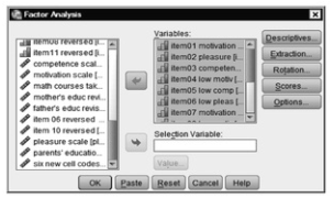
Fig.4.1.Factor analysis.

• Now click on .. to produce Fig. 4.2.
• Then click on the following: Initial solution and Univariate Descriptives (under Statistics), Coefficients, Determinant, and KMO and Bartlett’s test of sphericity (under Correlation Matrix).
• Click on Continue to return to 4.1.

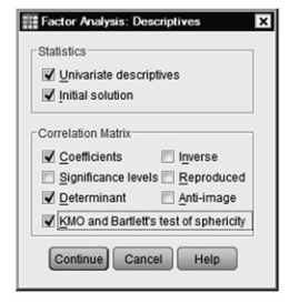
Fig.4.2. Factor analysis: Descriptives.

• Next, click on .. This will give you Fig. 4.3.
• Select Principal axis factoring from the Method pull-down menu.
• Unclick Unrotated factor solution (under Display). We will examine this only in Problem 4.2. We also usually would check the Scree plot However, again, we will request and interpret the scree plot only in 42.
• Click on Fixed number of factors under Extract, and type 3 in the box. This setting instructs the computer to extract three math attitude factors.
• Click on Continue to return to 4.1.

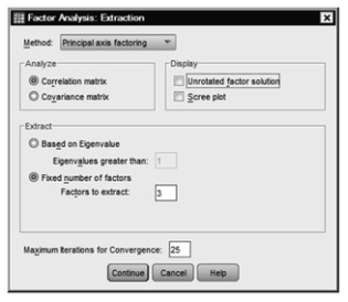
Fig. 4.3. Extraction method to produce principal axis factoring.

• Now click on .. in Fig. 4.1, which will give you Fig. 4.4.
• Click on Varimax, then make sure Rotated solution is also checked. Varimax rotation creates a solution in which the factors are orthogonal (uncorrelated with one another), which can make results easier to interpret and to replicate with future samples. If you believe that the factors (latent concepts) are correlated, you could choose Direct Oblimin, which will provide an oblique solution allowing the factors to be correlated.
• Click on Continue.

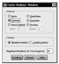
Fig.4.4.Factor analysis: Rotation.

• Next, click on Options. which will give you 4.5.
• Click on Sorted by size.
• Click on Suppress small coefficients and type .3 (point 3) in the Absolute Value below box (see 4.5). Suppressing small factor loadings makes the output easier to read.
• Click on Continue then OK. Compare Output 4.1 with your output and syntax.

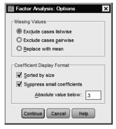
Fig.4.5.Factor analysis: Options.

Output 4.1: Factor Analysis for Math Attitude Questions

FACTOR

/VARIABLES item01 item02 item03 item04 item05 item06 item07 item08 item09 item10 item11 item12 item13 item14

/MISSING LISTWISE

/ANALYSIS item01 item02 item03 item04 item05 item06 item07 item08 item09 item10 item11 item12 item13 item14

/PRINT UNIVARIATE INITIAL CORRELATION DET KMO EXTRACTION ROTATION

/FORMAT SORT BLANK(.3)

/CRITERIA FACTORS(3) ITERATE(25)

/EXTRACTION PAF

/CRITERIA ITERATE(25)

/ROTATION VARIMAX

/METHOD=CORRELATION.

Factor Analysis

Interpretation of Output 4.1

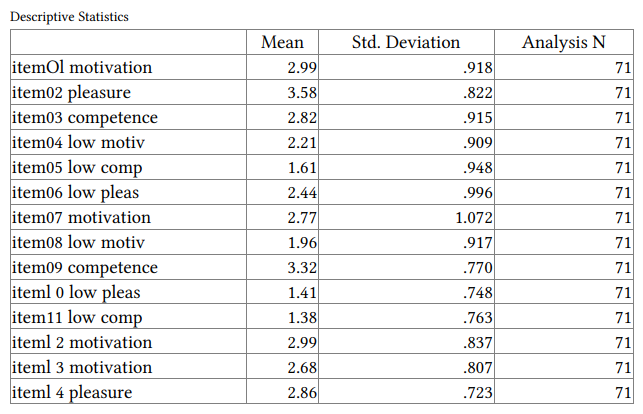
The factor analysis program generates a variety of tables depending on which options you have chosen. The first table includes Descriptive Statistics for each variable and the Analyses N, which in this case is 71 because several items have one or more participants missing. It is especially important to check the Analysis N when you have a small sample, scattered missing data, or one variable with lots of missing data. In the latter case, it may be wise to run the analysis without that variable.

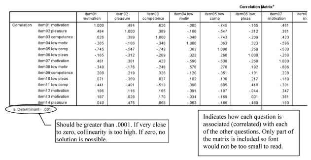
Indicates how each question is associated (correlated) with each of the other questions. Only part of the matrix is included so font would not be too small to read.

Interpretation of Output 4.1 continued The second table is part of a correlation matrix showing how each of the 14 items is associated with each of the other 13. Note that some of the correlations are high (e.g., + or -.60 or greater) and some are low (i.e., near zero). Relatively high correlations indicate that two items are associated and will probably be grouped together by the factor analysis. Items with low correlations (e.g., <.20) usually will not have high loadings on the same factor.

One assumption is that the determinant (located under the correlation matrix) should be more than .0001. Here, it is .001 so this assumption is met. If the determinant is zero, then a factor analytic solution cannot be obtained, because this would require dividing by zero, which would mean that at least one of the items can be understood as a linear combination of
some set of the other items.

Tests of assumptions.

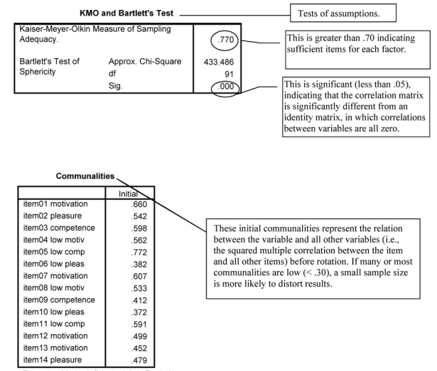
Interpretation of Output 4.1 continued The Kaiser-Meyer-Olkin (KMO) measure should be greater than .70 and is inadequate if less than .50. The KMO test tells us whether or not enough items are predicted by each factor. Here it is .77 so that is good. The Bartlett test should be significant (i.e., a significance value of less than .05); this means that the variables are correlated highly enough to provide a reasonable basis for factor analysis as in this case.

The Communalities table shows the Initial communalities before rotation. See the call out box for more interpretation. Note that all the initial communalities are above .30, which is good.

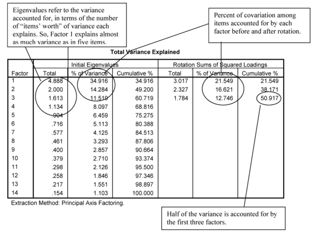
Interpretation of Output 4.1 continued The Total Variance Explained table shows how the variance is divided among the 14 possible factors. Note that four factors have eigenvalues (a measure of explained variance) greater than 1.0, which is a common criterion for a factor to be useful. When the eigenvalue is less than 1.0 the factor explains less information than a single item would have explained. Most researchers would not consider the information gained from such a factor to be sufficient to justify keeping that factor. Thus, if you had not specified otherwise, the computer would have looked for the best four-factor solution by “rotating” four factors. Because we specified that we wanted only three factors rotated, only three will be rotated, as seen on the
right side of the table under Rotation Sums of Squared Loadings.

For this and other analyses in this chapter, we will use an orthogonal rotation (varimax). This means that the final factors will be at right angles with each other. As a result, we can assume that the information explained by one factor is independent of the information in the other factors. Note that if we create scales by summing or averaging items with high loadings from each factor, these scales will not necessarily be uncorrelated; it is the best-fit vectors (factors) that are orthogonal.

Factor Matrix?

a- 3 factors extracted. 12 iterations required

Interpretation of Output 4.1 continued Factors are rotated so that they are easier to interpret.

Rotation makes it so that, as much as possible, different items are explained or predicted by different underlying factors, and each factor explains more than one item. This is a condition called simple structure. Although this is the goal of rotation, in reality, this is not always achieved. One thing to look for in the Rotated Matrix of factor loadings is the extent to which simple structure is achieved.

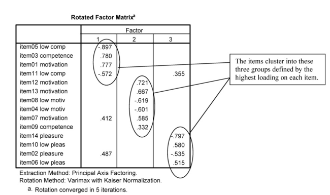
The Rotated Factor Matrix table is key for understanding the results of the analysis. Factors are rotated so that they are easier to interpret. Rotation makes it so that, as much as possible, different items are explained or predicted by different underlying factors, and each factor explains more than one item. This is a condition called simple structure. Although this is the goal of rotation, in reality, this is not always achieved. One thing to look for in the Rotated Matrix of factor loadings is the extent to which simple structure is achieved.

Note that the analysis has sorted the 14 math attitude questions (item01 to item14) into three somewhat overlapping groups of items, as shown by the circled items. The items are sorted so that the items that have the highest loading (not considering whether the correlation is positive or negative) from factor 1 (four items in this analysis) are listed first, and they are sorted from the one with the highest factor weight or loading (i.e., item05, with a loading of -.897) to the one with the lowest loading from that first factor (item11). Actually, every item has some loading from every factor, but we requested for loadings less than |.30| to be excluded from the output, so there are blanks where low loadings exist. (|.30| means the absolute value, or value without considering the sign.) Next, the six items that have their highest loading from factor 2 are listed from highest loading (item12) to lowest (item9). Finally, the four items on which factor 3 loads most highly are listed in order. Loadings resulting from an orthogonal rotation are correlation coefficients between each item and the factor, so they range from -1.0 through 0 to + 1.0. A negative loading just means that the question needs to be interpreted in the opposite direction from the way it is written for that factor (e.g., item05 “I am a little slow catching on to new topics in math” has a negative loading from the competence factor, which indicates that the people scoring higher on this item are lower in competence). Usually, factor loadings lower than |.30| are considered low, which is why we suppressed loadings less than |.30|. On the other hand, loadings of |.40| or greater are typically considered high. This is just a guideline, however, and one could set the criterion for “high” loadings as low as .30 or as high as .50. Setting the criterion lower than .30 or higher than .50 would be very unusual.

The investigator should examine the content of the items that have high loadings from each factor to see if they fit together conceptually and can be
named. Items 5, 3, and 11 were intended to reflect a perception of competence at math, so the fact that they all have strong loadings from the same factor provides some support for their being conceptualized as pertaining to the same construct. On the other hand, item01 was intended to measure motivation for doing math, but it is highly related to this same competence factor. In retrospect, one can see why this item could also be interpreted as competence. The item reads, “I practice math skills until I can do them well.” Unless one felt one could do math problems well, this would not be true. Likewise, item02, “I feel happy after solving a hard problem,” although intended to measure pleasure at doing math (and having its strongest loading there), might also reflect competence at doing math, in that, again, one could not endorse this item unless one had solved hard problems, which one could only do if one were good at math. Note that item02 loaded almost as highly (.49) on the competence factor (#1) as on the low pleasure factor (#3) so it loaded highly on two factors. On the other hand, item09, which was originally conceptualized as a competence item, had no really strong loadings.

Every item has a weight or loading from every factor, but in a “clean” factor analysis almost all of the loadings that are not in the circles that we have drawn on the Rotated Factor Matrix will be low (blank or less than |.40|). The fact that both Factors 1 and 3 load highly on item02 and fairly highly on item11, and the fact that Factors 1 and 2 both load highly on item07 is common but undesirable, in that one wants only one factor to predict each item.

Example of How to Write About Problem 4.1

Results

Principal axis factor analysis with varimax rotation was conducted to assess the underlying structure for the 14 items of the Math Attitude Questionnaire. (The assumption of independent sampling was met. The assumptions of normality, linear relationships between pairs of variables, and the variables’ being correlated at a moderate level were checked.) Three factors were requested, based on the fact that the items were designed to index three constructs: motivation, competence, and pleasure. After rotation, the first factor accounted for 21.5% of the variance, the second factor accounted for 16.6%, and the third factor accounted for 12.7%. Table 4.1 displays the items and factor loadings for the rotated factors, with loadings less than .40 omitted to improve clarity.

The first factor, which seems to index competence, had strong loadings on the first four items. Two of the items indexed low competence and had negative loadings. The second factor, which seemed to index motivation, had high loadings on the next five items in Table 4.1. “I prefer to figure out the problem without help” had its highest loading from the second factor but had a cross­loading over .4 on the competence factor. The third factor, which seemed to index low pleasure from math, loaded highly on the last four items in the table. “I feel happy after solving a hard problem” had its highest loading from the pleasure factor but also had a strong loading from the competence factor.

Source: Leech Nancy L. (2014), IBM SPSS for Intermediate Statistics, Routledge; 5th edition;

download Datasets and Materials.