Problem 4.3: Boxplots and Stem-and-Leaf Plots Split by a Dichotomous Variable with SPSS

Now let’s make a boxplot comparing males and females on math achievement. This is similar to what we did in Chapter 3, but here we request statistics and stem-and-leaf plots.

4.3. Create a boxplot for math achievement split by gender.

Use these commands:

• Analyze → Descriptive Statistics → Explore 
• The Explore window (Fig. 4.5) will appear.
• Click on math achievement and move it to the Dependent List.
• Next, click on gender and move it to the Factor (or independent variable)
• Click on Both under This will produce both a table of descriptive statistics and two kinds of plots: stem-and-leaf and box-and-whiskers.

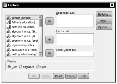
Fig. 4.5. Explore.

• Click on OK.

You will get an output file complete with syntax, statistics, stem-and-leaf plots, and boxplots. See Output 4.3 and compare it to your own output and syntax. As with most SPSS procedures, we could have requested a wide variety of other statistics if we had clicked on Statistics and/or Plots in Fig 4.5.

Output 4.3: Boxplots Split by Gender With Statistics and Stem-and-Leaf Plots

EXAMINE VARIABLES=mathach BY gender

/PLOT BOXPLOT STEMLEAF

/COMPARE GROUP

/STATISTICS DESCRIPTIVES

/CINTERVAL 95

/MISSING LISTWISE

/NOTOTAL.

Explore

Gender

math achievement test
Stem-and-Leaf Plots

Interpretation of Output 4.3

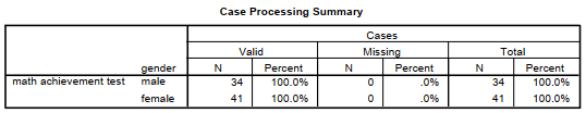
The first table under Explore provides descriptive statistics about the number of males and females with Valid and Missing data. Note that we have 34 males and 41 females with valid math achievement test scores.

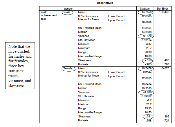
The Descriptives table contains many different statistics for males and females separately. Several of them are beyond what we cover in this book. Note that the average math achievement test score is 14.76 for males and 10.75 for females. We discuss the variances and skewness below under assumptions.

The Stem-and-Leaf Plots for each gender separately are next. These plots are like a histogram or frequency distribution turned on the side. They give a visual impression of the distribution, and they show each person’s score on the dependent variable (math achievement). Note that the legend indicates that Stem width equals 10 and Each leaf equals one case. This means that entries that have 0 for the stem are less than 10, those with 1 as the stem range from 10 to 19, and so forth. Each number in the Leaf column represents the last digit of one person’s math achievement score. The numbers in the Frequency column indicate how many participants had scores in the range represented by that stem and range of leaves. Thus, in the male plot, one student had a Stem of 0 and a Leaf of 3, that is, a score of 03 (or 3). The Frequency of students with leaves between 05 and 09 is 7, and there were three scores of 5, two of 7, and two of 9. One had a Stem of 1 and a Leaf of 0 (a score of 10); two had scores of 11, and so forth.

Boxplots are the last part of the output. This figure has two boxplots (one for males and one for females). By inspecting the plots, we can see that the median score for males is quite a bit higher than that for females, although there is substantial overlap of the boxplots, with the highest female score equaling the highest male score. We therefore need to be careful in concluding that males score higher than females, especially based on a small sample of students. In Chapter 9, we show how an inferential statistic (the t test) can help us know how likely it is that this apparent difference could have occurred by chance.

Using the output to check your data for errors. Checking the box and stem-and-leaf plots can help identify outliers that might be data entry errors. In this case there aren’t any.

Using the output to check your data for assumptions. As noted in the interpretation of

Outputs 4.2a and 4.2b, you can tell if a variable is grossly non-normal by looking at the boxplots. The stem-and-leaf plots provide similar information. You can also examine the skewness values for each gender separately in the table of Descriptives (see the circled skewness values). Note that for both males and females, the skewness values are less than one, which indicates that math achievement is approximately normal for both genders. This is an assumption of the t test.

The Descriptives table also provides the variances for males and females. A key assumption of the t test is that the variances are approximately equal (i.e., the assumption of homogeneity of variances). Note that the variance is 36.38 for males and 44.84 for females. These do not seem grossly different, and we find out in Chapter 9 that they are, in fact, not significantly different. Thus, the assumption of homogeneous variances is not violated.

Source: Morgan George A, Leech Nancy L., Gloeckner Gene W., Barrett Karen C.

(2012), IBM SPSS for Introductory Statistics: Use and Interpretation, Routledge; 5th edition; download Datasets and Materials.