Problem 9.3: Analyses of Covariance (ANCOVA) with SPSS

ANCOVA is an extension of ANOVA that typically provides a way of statistically controlling for the effects of continuous or scale variables that you are concerned about but that are not the focal point or independent variable(s) in the study. These continuous variables are called covariates (or sometimes, control variables). Covariates usually are variables that may cause you to draw incorrect inferences about the prediction of the dependent variable from the independent variable, if not controlled (then are possible confounds). It is also possible to use ANCOVA when you are interested in examining a combination of a categorical (nominal) variable and a continuous (scale) variable as predictors of the dependent variable. In this latter case, you would not consider the covariate to be an extraneous variable but rather a variable that is of interest in the study. SPSS will allow you to determine the significance of the contribution of the covariate as well as whether the nominal variables (factors) significantly predict the dependent variable, over and above the “effect” of the covariate.

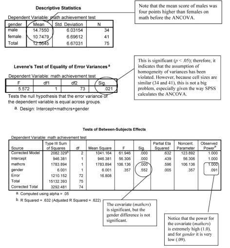
In the HSB data, boys have significantly higher math achievement scores than girls. To see if the males’ higher math achievement scores are due to differences in the number of math courses taken by the male and female students, we will use math courses taken as a covariate and do ANCOVA.

9.3 Do boys have higher math achievement than girls if we control for

differences in the number of math courses taken?

To answer this question, first, we need to assess the assumption of homogeneity of regression slopes:

• Analyze → General Linear Model → Univariate.
• Next, move math achievement to the Dependent box, gender to the Fixed Factor box, and math courses taken to the Covariates box (see 9.12).

Fig. 9.12. GLM: Univariate.

• Click on Model and then click on the button next to Custom under

Specify Model (see Fig. 9.13).

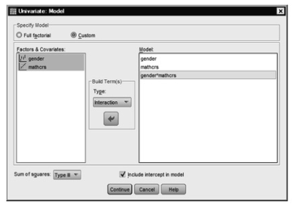
Fig. 9.13. Univariate: Model.

• Move gender from the Factor & Covariates box to the Model Do the same for mathcrs.
• Next highlight gender again, but hold down the “Shift” key and highlight mathcrs. This will allow you to have both gender and mathcrs highlighted at the same time. Click on the arrow to move both variables together to the Model This will make gender*mathcrs.
• Click on Continue and then OK. Your syntax and output should look like the beginning of Output 9.3.

Next, do the following:

• Analyze → General Linear Model → Univariate.
• Click on Reset.
• Next, move math achievement to the Dependent box, gender to the Fixed Factor box, and math courses taken to the Covariates box (see 9.12).
• Click on Options to get 9.14.

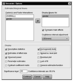
Fig. 9.14. GLM: Univariate options.

• Select Descriptive statistics, Estimates of effect size, Observed power, and Homogeneity tests.
• Move gender into the box labeled Display Means for (see 9.14).
• Click on Compare main effects to include output that will show which levels are statistically significantly different from one another.
• Be sure LSD(none) is in the Confidence interval adjustment pull-down menu.
• Click on Continue and then OK. Your syntax and output should look like the rest of Output 9.3.

Output 9.3: Analysis of Covariance (ANCOVA)

UNIANOVA mathach BY gender WITH mathcrs /METHOD = SSTYPE(3)

/INTERCEPT = INCLUDE

/CRITERIA = ALPHA(.05)

/DESIGN = gender mathcrs gender*mathcrs.

Univariate Analysis of Variance

UNIANOVA mathach BY gender WITH mathcrs

/METHOD = SSTYPE(3)

/INTERCEPT = INCLUDE

/EMMEANS = TABLES(gender) WITH(mathcrs=MEAN)

/PRINT = DESCRIPTIVE ETASQ OPOWER HOMOGENEITY

/CRITERIA = ALPHA(.05)

/DESIGN = mathcrs gender.

Univariate Analysis of Variance

Interpretation of Output 9.3

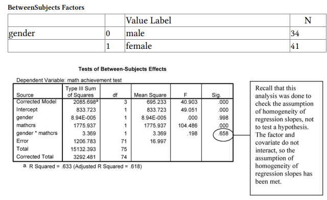
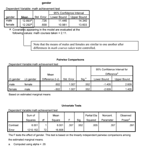
The ANCOVA (Tests of BetweenSubject Effects) table is interpreted in much the same way as ANOVA tables in earlier outputs. The covariate (mathcrs) has a highly significant “effect” on math achievement, as should be the case. However, the “effect” of gender is no longer significant, F(1,72) = .36, p = .55. You can see from the Estimated Marginal Means table that the statistically adjusted math achievement means for boys and girls are quite similar once differences in the number of math courses taken were accounted for. This suggests that the fact that males took more math courses may have been the reason for their higher math achievement.

The Observed Power for math courses taken was 1.0, which indicates extremely high power. For gender the observed power was .091. This is very low power. The effect size for gender is also very small (partial eta = .071), so it may be that we have overlooked an important gender difference because of this low power. It is possible that once the strong relation between the number of math courses taken and math achievement was taken into account, there was no longer an important “effect” of gender on math achievement.

We include the Pairwise Comparisons table to show how to produce a post hoc test for the multiple levels of the independent variable. In our example, this table is not helpful since our overall test was not significant. If we had found a significant difference among an independent variable that had three or more levels, the Pairwise Comparison table would show which levels were significantly different from one another. We would also need to calculate an effect size (i.e., Cohen’s d) for each pair that was statistically significantly different. To do so, we need to calculate the standard deviation for the estimated marginal means by using the formula: SD = SE(Tn). We would use this standard deviation and the new estimated marginal means to calculate Cohen’s d.

The Univariate Test table can be ignored since it gives us the same information as the Tests of BetweenSubject Effects table.

Example of How to Write About Problems 9.3

Results

An analysis of covariance was used to assess whether boys have higher math achievement than girls after controlling for differences between boys and girls in the number of math courses taken (Table 9.6). (The following assumptions were checked, (a) independence of observations, (b) normal distribution of the dependent variable, (c) homogeneity of variances, (d) linear relationships between the covariates and the dependent variable, and (e) homogeneity of regression slopes. The assumption of homogeneity of variances was violated; however, because cell sizes were similar (34 and 41), this violation did not present an issue. All other assumptions were met.) Results indicate that after controlling for the number of math courses taken, there is not a significant difference between boys and girls in math achievement, F( 1, 72) = .36, p = .552, partial eta² = .01. Table 9.5 presents the means and standard deviations for boys and girls on math achievement before and after controlling for number of math courses taken. As is evident from this table, virtually no difference between boys and girls remains after differences in number of math courses taken are controlled.

Source: Leech Nancy L. (2014), IBM SPSS for Intermediate Statistics, Routledge; 5th edition;

download Datasets and Materials.