Performing the regression analysis computations without the help of a computer can be quite time consuming. In this section we discuss how the computational burden can be minimized by using a computer software package such as JMP or Excel.
Although the layout of the information may differ by computer software, the information shown in Figure 14.10 is fairly typical. We will use the structure illustrated in Figure 14.10 but be aware that the particular package you use may differ in style and in number of digits shown in the numerical output.
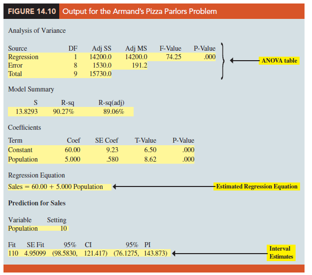
We have highlighted the portions of the output that are topics we have previously discussed in this chapter (the portions of the output not highlighted are beyond the scope of this text, but can be found in more advanced statistics texts).
The interpretation of the highlighted portion of the printout follows.
- The ANOVA table is printed below the heading Analysis of Variance. The label Error is used for the error source of variation. Note that DF is an abbreviation for degrees of freedom and that MSR is given in the Regression row under the column Adj MS as 14,200 and MSE is given in the Error row under Adj MS as 191.2. The ratio of these two values provides the F value of 74.25 and the corresponding p-value of .000. Because the p-value is zero (to three decimal places), the relationship between Sales and Population is judged statistically significant.
- Under the heading Model Summary, the standard error of the estimate, 5 = 13.8293, is given as well as information about the goodness of fit. Note that “R-sq = 90.27%” is the coefficient of determination expressed as a percentage. The value “R-Sq(adj) = 89.06%” is discussed in Chapter 15.
- A table is printed that shows the values of the coefficients b0 and b1, the standard deviation of each coefficient, the t value obtained by dividing each coefficient value by its standard deviation, and the p-value associated with the t This appears under the heading Coefficients. Because the p-value is zero (to three decimal places), the sample results indicate that the null hypothesis (H0: b1 = 0) should be rejected. Alternatively, we could compare 8.62 (located in the T-Value column) to the appropriate critical value. This procedure for the t test was described in Section 14.5.
- Under the heading Regression Equation, the estimated regression equation is given: Sales = 60.00 + 5.000 Population.
- The 95% confidence interval estimate of the expected sales and the 95% prediction interval estimate of sales for an individual restaurant located near a campus with 10,000 students are printed below the ANOVA table. The confidence interval is (98.5830, 121.4417) and the prediction interval is (76.1275, 143.873) as we showed in Section 14.6.
Source: Anderson David R., Sweeney Dennis J., Williams Thomas A. (2019), Statistics for Business & Economics, Cengage Learning; 14th edition.
There is noticeably a bundle to know about this. I assume you made certain nice points in features also.