The sample proportion p is the point estimator of the population proportion p. The formula for computing the sample proportion is
![]()
where
x = the number of elements in the sample that possess the characteristic of interest
n = sample size
As noted in Section 7.4, the sample proportion p is a random variable and its probability distribution is called the sampling distribution of p.
To determine how close the sample proportion p is to the population proportion p, we need to understand the properties of the sampling distribution of p: the expected value of p, the standard deviation of p, and the shape or form of the sampling distribution of p.
1. Expected Value of p
The expected value of p, the mean of all possible values of p, is equal to the population proportion p.

Because E(p) = p, p is an unbiased estimator of p. Recall from Section 7.1 we noted that p = .60 for the EAI population, where p is the proportion of the population of managers who participated in the company’s management training program. Thus, the expected value of p for the EAI sampling problem is .60.
2. Standard Deviation of p
Just as we found for the standard deviation of X, the standard deviation of p depends on whether the population is finite or infinite. The two formulas for computing the standard deviation of p follow.

Comparing the two formulas in (7.5), we see that the only difference is the use of the finite population correction factor ![]()
As was the case with the sample mean X, the difference between the expressions for the finite population and the infinite population becomes negligible if the size of the finite population is large in comparison to the sample size. We follow the same rule of thumb that we recommended for the sample mean. That is, if the population is finite with n/N < .05, we will use ![]() However, if the population is finite with n/N > .05, the finite population correction factor should be used. Again, unless specifically noted, throughout the text we will assume that the population size is large in relation to the sample size and thus the finite population correction factor is unnecessary.
However, if the population is finite with n/N > .05, the finite population correction factor should be used. Again, unless specifically noted, throughout the text we will assume that the population size is large in relation to the sample size and thus the finite population correction factor is unnecessary.
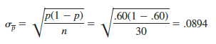
In Section 7.5 we used the term standard error of the mean to refer to the standard deviation of x. We stated that in general the term standard error refers to the standard deviation of a point estimator. Thus, for proportions we use standard error of the proportion to refer to the standard deviation of p. Let us now return to the EAI example and compute the standard error of the proportion associated with simple random samples of 30 EAI managers.
For the EAI study we know that the population proportion of managers who participated in the management training program is p = .60. With n/N = 30/2500 = .012, we can ignore the finite population correction factor when we compute the standard error of the proportion. For the simple random sample of 30 managers, σp is
3. Form of the Sampling Distribution of p
Now that we know the mean and standard deviation of the sampling distribution of p, the final step is to determine the form or shape of the sampling distribution. The sample proportion is p = x/n. For a simple random sample from a large population, the value of x is a binomial random variable indicating the number of elements in the sample with the characteristic of interest. Because n is a constant, the probability of x/n is the same as the binomial probability of x, which means that the sampling distribution of p is also a discrete probability distribution and that the probability for each value of x/n is the same as the probability of x.
In Chapter 6 we also showed that a binomial distribution can be approximated by a normal distribution whenever the sample size is large enough to satisfy the following two conditions:
![]()
Assuming these two conditions are satisfied, the probability distribution of x in the sample proportion, p = x/n, can be approximated by a normal distribution. And because n is a constant, the sampling distribution of p can also be approximated by a normal distribution. This approximation is stated as follows:
The sampling distribution of p can be approximated by a normal distribution whenever np ≥ 5 and n(1 – p) ≥ 5.
In practical applications, when an estimate of a population proportion is desired, we find that sample sizes are almost always large enough to permit the use of a normal approximation for the sampling distribution of p.
Recall that for the EAI sampling problem we know that the population proportion of managers who participated in the training program is p = .60. With a simple random sample of size 30, we have np = 30(.60) = 18 and n(1 – p) = 30(.40) = 12. Thus, the sampling distribution of p can be approximated by a normal distribution shown in Figure 7.8.
4. Practical Value of the Sampling Distribution of p
The practical value of the sampling distribution of p is that it can be used to provide probability information about the difference between the sample proportion and the population proportion. For instance, suppose that in the EAI problem the personnel director wants to know the probability of obtaining a value of p that is within .05 of the population proportion of EAI managers who participated in the training program. That is, what is the probability of obtaining a sample with a sample proportion p between .55 and .65? The darkly shaded area in Figure 7.9 shows this probability.

Using the fact that the sampling distribution of p can be approximated by a normal distribution with a mean of .60 and a standard error of the proportion of Sp = .0894, we find that the standard normal random variable corresponding to p = .65 has a value of z = (.65 – .60)/.0894 = .56. Referring to the standard normal probability table, we see that the cumulative probability corresponding to z = .56 is .7123. Similarly, at p = .55, we find z = (.55 – .60)/.0894 = -.56. From the standard normal probability table, we find the cumulative probability corresponding to z = -.56 is .2877. Thus, the probability of selecting a sample that provides a sample proportion p within .05 of the population proportion p is given by .7123 – .2877 = .4246.

If we consider increasing the sample size to n = 100, the standard error of the proportion becomes

With a sample size of 100 EAI managers, the probability of the sample proportion having a value within .05 of the population proportion can now be computed. Because the sampling distribution is approximately normal, with mean .60 and standard deviation .049, we can use the standard normal probability table to find the area or probability. At p = .65, we have z = (.65 – .60)/.049 = 1.02. Referring to the standard normal probability table, we see that the cumulative probability corresponding to z = 1.02 is .8461. Similarly, at p = .55, we have z = (.55 – .60)/.049 = -1.02. We find the cumulative probability corresponding to z = -1.02 is .1539. Thus, if the sample size is increased from 30 to 100, the probability that the sample proportion p is within .05 of the population proportion p will increase to .8461 – .1539 = .6922.
Source: Anderson David R., Sweeney Dennis J., Williams Thomas A. (2019), Statistics for Business & Economics, Cengage Learning; 14th edition.
28 Aug 2021
30 Aug 2021
30 Aug 2021
30 Aug 2021
30 Aug 2021
31 Aug 2021