Interaction Effects in Linear Regression by using Stata

The previous section described what are called “intercept dummy variables,” because their coefficients amount to shifts in a regression equation’s y intercept, comparing the 0 and 1 groups. Another use for dummy variables is to form interaction terms called “slope dummy variables” by multiplying a dummy times a measurement variable. In this section we stay with the Nations2.dta data, but consider some different variables: per capita carbon dioxide emissions (co2), percent of the population living in urban areas (urban), and the dummy variable reg4 defined as 1 for European countries and 0 for all others. We start out by labeling the values of reg4, and calculating a log version of co2 because of that variable’s severe positive skew.

We form an interaction term or slope dummy variable named urb_reg4 by multiplying the dummy variable reg4 times the measurement variable urban. The resulting variable urb_reg4 equals urban for countries in Europe, and zero for all other countries.

. generate urb_reg4 = urban * reg4

. label variable urb_reg4 “interaction urban*reg4 (Europe)”

Regressing logco2 on urban, reg4 and the interaction term urb_reg4 gives a model that tests whether either the y-intercept or the slope relating logco2 to urban might be different for Europe compared with other regions.

The interaction effect is statistically significant (p = .043), suggesting that the relationship between percent urban and log CO₂ emissions is different for Europe than for the rest of the world. The main effect of urban is positive (.0217), meaning that logco2 tends to be higher in countries with more urbanized population. But the interaction coefficient is negative, meaning that this upward slope is less steep for Europe. We could write the model above as two separate equations:

The post-regression command predict newvar generates a new variable holding predicted values from the recent regression. Graphing the predicted values for this example visualizes our interaction effect (Figure 7.7). The line in the left-hand (reg4 = 0) panel has a slope of .0217 and y-intercept -.4682. The line in the right panel (reg4 = 1) has a less-steep slope (.0084) and a higher y-intercept (.826). No European countries exhibit the low-urbanization, low-CO₂ profile seen in other parts of the world; and even European nations with middling urbanization have relatively high CO₂ emissions.

. predict co2hat

. graph twoway scatter logco2 urban, msymbol(Oh)

|| connect co2hat urban, msymbol(+)

|| , by(reg4)

The i.varname and c.varname notation for indicator and continuous variables, introduced in Chapter 6, provides an alternative way to include interactions. The symbol # specifies an interaction between two variables, and ## a factorial interaction which automatically includes all the lower-level interactions involving those variables. reg4 is an indicator variable and urban is continuous, so the same model estimated above could be obtained by the command

. regress logco2 c.urban i.reg4 c.urban#i.reg4

or equivalently with a factor interaction,

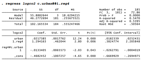
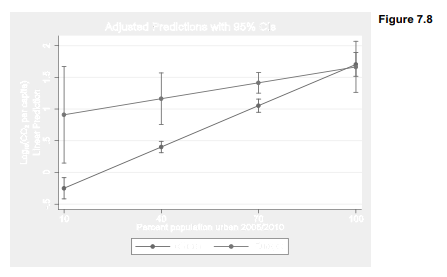
margins understands # or ## interactions. Percent urban ranges from about 10 to 100 percent in these data, so we could graph the interaction as follows. First calculate the predicted means of logco2 at several combinations of urban (10, 40, 70 or 100) and reg4 (0 or 1).

Next, use marginsplot to graph these means. Note the use of twoway-type options to label details of the graph. Figure 7.8 visualizes the same model as Figure 7.7, but in a different style that shows confidence intervals for the predicted means instead of data points. The option in the following marginsplot command specifies l2 (letter “el” 2), a second left-hand axis title.

. marginsplot, l2(“Log{subscript:10}(CO{subscript:2} per capita)”) xlabel(10(30)100)

Interaction effects could also involve two measurement variables. A trick called centering helps to reduce multicollinearity problems with such interactions, and makes their main effects easier to interpret. Centering involves subtracting their respective means from both variables before defining an interaction term as their product. Centered variables have means approximately equal to zero, and are negative for below-average values. The commands below calculate centered versions of urban and loggdp, named urbanO and loggdpO. The interaction term urb_gdp is then defined as the product of urbanO times loggdpO.

More precise centering could be performed using means returned by summarize:

. summarize urban

. generate urbanOO = urban – r(mean)

We might also set aside all observations with missing values on any variables in the regression, before obtaining a mean for centering.

Regressing logco2 on the centered main effects loggdpO and urbanO, along with the interaction term urb_gdp, we find that the interaction effect is negative and statistically significant.

The same regression could have been conducted, and the continuous-by-continuous variable interaction effect graphed, with the following three commands (results not shown).

. regress logco2 c.loggdpO c.urbanO c.loggdp0#c.urbanO

. margins, at(loggdpO = (-1.3 1.1) urbanO = ( -45 45))

. marginsplot

Main effects in a regression of this sort, where the interacting variables have been centered, can be interpreted as the effect of each variable when the other is at its mean. Thus, predicted logco2 rises by 1.12 with each 1-unit increase in loggdp, when urban is at its mean. Similarly, predicted logco2 rises by only a small amount, .0025, with each 1-unit increase in urban when loggdp is at its mean. The coefficient on interaction term urb_gdp, however, tells us that with each 1-unit increase in urbanization, the effect of loggdp on logco2 becomes weaker, decreasing by -.008. That is, CO₂ emissions increase as wealth increases, but do so less steeply in more urbanized countries.

Source: Hamilton Lawrence C. (2012), Statistics with STATA: Version 12, Cengage Learning; 8th edition.