Uniform Probability Distribution

Consider the random variable x representing the flight time of an airplane traveling from Chicago to New York. Suppose the flight time can be any value in the interval from 120 minutes to 140 minutes. Because the random variable x can assume any value in that interval, x is a continuous rather than a discrete random variable. Let us assume that sufficient actual flight data are available to conclude that the probability of a flight time within any 1-minute interval is the same as the probability of a flight time within any other 1-minute interval contained in the larger interval from 120 to 140 minutes. With every 1-minute interval being equally likely, the random variable x is said to have a uniform probability distribution. The probability density function, which defines the uniform distribution for the flight-time random variable, is

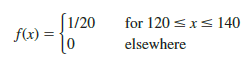
Figure 6.1 is a graph of this probability density function. In general, the uniform proba­bility density function for a random variable x is defined by the following formula.

For the flight-time random variable, a = 120 and b = 140.

As noted in the introduction, for a continuous random variable, we consider proba­bility only in terms of the likelihood that a random variable assumes a value within a specified interval. In the flight time example, an acceptable probability question is: What is the probability that the flight time is between 120 and 130 minutes?

That is, what is P(120 < x < 130)? Because the flight time must be between 120 and 140 minutes and because the probability is described as being uniform over this interval, we feel comfortable saying P(120 < x < 130) = .50. In the following subsection we show that this probability can be computed as the area under the graph off(x) from 120 to 130 (see Figure 6.2).

Area as a Measure of Probability

Let us make an observation about the graph in Figure 6.2. Consider the area under the graph of f(x) in the interval from 120 to 130. The area is rectangular, and the area of a rectangle is simply the width multiplied by the height. With the width of the interval equal to 130 – 120 = 10 and the height equal to the value of the probability density function f(x) = 1/20, we have area = width X height = 10(1/20) = 10/20 = .50.

What observation can you make about the area under the graph of f(x) and probability? They are identical! Indeed, this observation is valid for all continuous random variables. Once a probability density function f (x) is identified, the probability that x takes a value between some lower value x₁ and some higher value x₂ can be found by computing the area under the graph of f(x) over the interval from x₁ to x₂.

Given the uniform distribution for flight time and using the interpretation of area as probability, we can answer any number of probability questions about flight times. For example, what is the probability of a flight time between 128 and 136 minutes? The width of the interval is 136 – 128 = 8. With the uniform height of f(x) = 1/20, we see that P(128 < x < 136) = 8(1/20) = .40.

Note that P(120 < x < 140) = 20(1/20) = 1; that is, the total area under the graph of fix) is equal to 1. This property holds for all continuous probability distributions and is the analog of the condition that the sum of the probabilities must equal 1 for a discrete prob­ability function. For a continuous probability density function, we must also require that fix) > 0 for all values of x. This requirement is the analog of the requirement that fix) > 0 for discrete probability functions.

Two major differences stand out between the treatment of continuous random variables and the treatment of their discrete counterparts.

1. We no longer talk about the probability of the random variable assuming a particu­lar value. Instead, we talk about the probability of the random variable assuming a value within some given interval.
2. The probability of a continuous random variable assuming a value within some given interval from x₁ to x₂ is defined to be the area under the graph of the probabil­ity density function between x₁ and x₂. Because a single point is an interval of zero width, this implies that the probability of a continuous random variable assuming any particular value exactly is zero. It also means that the probability of a continu­ous random variable assuming a value in any interval is the same whether or not the endpoints are included.

The calculation of the expected value and variance for a continuous random variable is analogous to that for a discrete random variable. However, because the computational procedure involves integral calculus, we leave the derivation of the appropriate formulas to more advanced texts.

For the uniform continuous probability distribution introduced in this section, the for­mulas for the expected value and variance are

In these formulas, a is the smallest value and b is the largest value that the random variable may assume.

Applying these formulas to the uniform distribution for flight times from Chicago to New York, we obtain

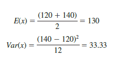
The standard deviation of flight times can be found by taking the square root of the variance. Thus, s = 5.77 minutes

Source:  Anderson David R., Sweeney Dennis J., Williams Thomas A. (2019), Statistics for Business & Economics, Cengage Learning; 14th edition.