How can the inefficiency resulting from an externality be remedied? If the firm that generates the externality has a fixed-proportions production technology, the externality can be reduced only by encouraging the firm to produce less. As we saw in Chapter 8, this goal can be achieved through an output tax. Fortunately, most firms can substitute among inputs in the production process by altering their choices of technology. For example, a manufacturer can add a scrubber to its smokestack to reduce emissions.
Consider a firm that sells its output in a competitive market. The firm emits pollutants that damage air quality in a neighborhood. The firm can reduce its emissions, but only at a cost. Figure 18.4 illustrates this trade-off. The horizontal axis represents the level of factory emissions and the vertical axis the cost per unit of emissions. To simplify, we assume that the firm’s output decision and its emissions decision are independent and that the firm has already chosen its profit-maximizing output level. The firm is therefore ready to choose its preferred level of emissions. The curve labeled MEC represents the marginal external cost of emissions. This social cost curve represents the increased harm associated with the emissions. We will use the terms marginal external cost and marginal social cost interchangeably in the discussion that follows. (Recall that we have assumed that the firm’s output is fixed, so that the private costs of production—as opposed to pollution abatement—are unchanged.) The MEC curve slopes upward because the marginal cost of the externality gets higher as the externality becomes more extensive. (Evidence from studies of the effects of air and water pollution suggests that small levels of pollutants generate little harm. However, the harm increases substantially as the level of pollutants increases.)
Because our emphasis will be on reducing emissions from existing levels, we will find it useful to read the MEC graph from right to left. From this perspective, we see that the MEC associated with a small reduction in emissions from a level of 26 units, which reflects the incremental benefit of reduced emissions, is greater than $6 per unit. However, as emissions are reduced further and further, the marginal social cost falls (eventually) to below $2 per unit. At some point, the incremental benefit of reducing emissions becomes less than $2.
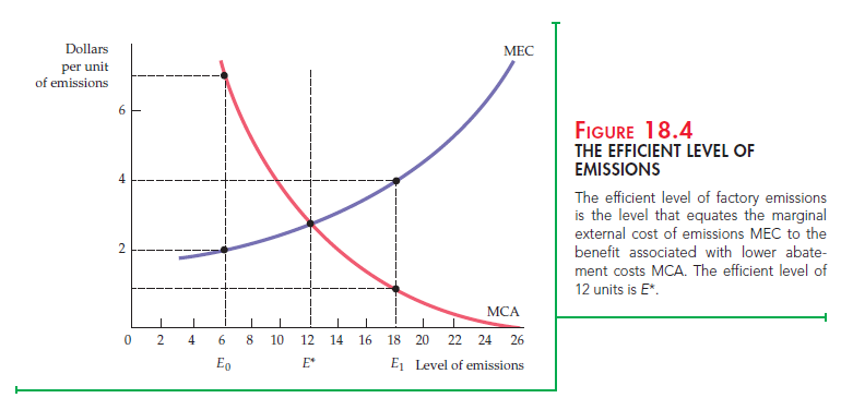
The curve labeled MCA is the marginal cost of abating emissions. It measures the additional cost to the firm of installing pollution-control equipment. The MCA curve is downward sloping because the marginal cost of reducing emissions is low when the reduction has been slight and high when it has been substantial. (A slight reduction is inexpensive—the firm can reschedule production to generate the greatest emissions at night, when few people are outside. Large reductions require costly changes in the production process.) As with the MEC curve, reading the MCA curve from right to left will help with our intuition. From this perspective, the marginal cost of abatement increases as we seek to achieve greater and greater reductions in emissions.
With no effort at abatement, the firm’s profit-maximizing level of emissions is 26, the level at which the marginal cost of abatement is zero. The efficient level of emissions, 12 units, is at point E*, where the marginal external cost of emissions, $3, is equal to the marginal cost of abating emissions. Note that if emissions are lower than E*—say, E0—the marginal cost of abating emissions, $7, is greater than the marginal external cost of emissions, $2. Emissions, therefore, are too low relative to the social optimum. However, if the level of emissions is E1, the marginal external cost of emissions, $4, is greater than the marginal cost of abatement, $1. Emissions are then too high.
We can encourage the firm to reduce emissions to E* in three ways: (1) emissions standards; (2) emissions fees; and (3) transferable emissions permits. We will begin by discussing standards and fees and comparing relative advantages and disadvantages. Then we will examine transferable emissions permits.
1. An Emissions Standard
An emissions standard is a legal limit on how much pollutant a firm can emit. If the firm exceeds the limit, it can face monetary and even criminal penalties. In Figure 18.5, the efficient emissions standard is 12 units, at point E*. The firm will be heavily penalized for emissions greater than this level.
The standard ensures that the firm produces efficiently. The firm meets the standard by installing pollution-abatement equipment. The increased abatement expenditure will cause the firm’s average cost curve to rise (by the average cost of abatement). Firms will find it profitable to enter the industry only if the price of the product is greater than the average cost of production plus abate- ment—the efficient condition for the industry.
2. An Emissions Fee
An emissions fee is a charge levied on each unit of a firm’s emissions. As Figure 18.5 shows, a $3 emissions fee will generate efficient behavior by our factory. Faced with this fee, the firm minimizes costs by reducing emissions from 26 to 12 units. To see why, note that the first unit of emissions can be reduced (from 26 to 25 units of emissions) at very little cost (the marginal cost of additional abatement is close to zero). For very little cost, therefore, the firm can avoid paying the $3 per-unit fee. In fact, for all levels of emissions above 12 units, the marginal cost of abatement is less than the emissions fee. Thus it pays to reduce emissions. Below 12 units, however, the marginal cost of abatement is greater than the fee. In that case, the firm will prefer to pay the fee rather than further reduce emissions. It will therefore pay a total fee given by the gray-shaded rectangle and incur a total abatement cost given by the blue-shaded triangle under the MCA curve to the right of E = 12. This cost is less than the fee that the firm would pay if it did not reduce emissions at all.

3. Standards versus Fees
The United States has historically relied on standards to regulate emissions. However, other countries, such as Germany, have used fees successfully. Which method is better? The relative advantages of standards and fees depend on the amount of information available to policymakers and on the actual cost of controlling emissions. To understand these differences, let’s suppose that because of administrative costs, the agency that regulates emissions must charge the same fee or set the same standard for all firms.
THE CASE FOR FEES First, let’s examine the case for fees. Consider two firms that are located so that the marginal social cost of emissions is the same no matter which reduces its emissions. Because they have different abatement costs, however, their marginal cost of abatement curves are not the same. Figure 18.6 shows why emissions fees are preferable to standards in this case. MCA1 and MCA2 represent the marginal cost of abatement curves for the two firms. Each firm initially generates 14 units of emissions. Suppose we want to reduce total emissions by 14 units. Figure 18.6 shows that the cheapest way to do this is to have Firm 1 reduce emissions by 6 units and Firm 2 by 8. With these reductions, both firms have marginal costs of abatement of $3. But consider what happens if the regulatory agency asks both firms to reduce emissions by 7 units. In that case Firm 1’s marginal cost of abatement increases from $3 to $3.75, while Firm 2’s marginal cost of abatement decreases from $3 to $2.50. This cannot be cost-minimizing because the second firm can reduce emissions more cheaply than the first. Only when the marginal cost of abatement is equal for both firms will emissions be reduced by 14 units at minimum cost.
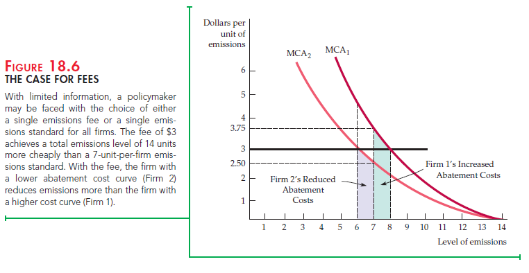
Now we can see why a fee ($3) might be preferable to a standard (7 units). Faced with a $3 fee, Firm 1 will reduce emissions by 6 units and Firm 2 by 8 units—the efficient outcome. By contrast, under an emissions standard, Firm 1 incurs additional abatement costs given by the green-shaded area between 7 and 8 units of emissions. But Firm 2 enjoys reduced abatement costs given by the purple-shaded area between 6 and 7 units. Clearly, Firm 1’s added abatement costs are larger than Firm 2’s reduced costs. The emissions fee thus achieves the same level of emissions at a lower cost than the equal per-firm emissions standard.
In general, fees can be preferable to standards for several reasons. First, when standards must be applied equally to all firms, fees achieve the same emissions reduction at a lower cost. Second, fees give a firm a strong incentive to install new equipment that would allow it to reduce emissions even further. Suppose the standard requires that each firm reduce its emission by 6 units, from 14 to 8. Firm 1 is considering installing new emissions devices that would lower its marginal cost of abatement from MCA1 to MCA2. If the equipment is relatively inexpensive, the firm will install it because it will lower the cost of meeting the standard. However, a $3 emissions fee would provide a greater incentive for the firm to reduce emissions. With the fee, not only will the firm’s cost of abatement be lower on the first 6 units of reduction, but it will also be cheaper to reduce emissions by 2 more units: The emissions fee is greater than the marginal abatement cost for emissions levels between 6 and 8.
THE CASE FOR STANDARDS Now let’s examine the case for standards by looking at Figure 18.7. While the marginal external cost curve is very steep, the marginal cost of abatement is relatively flat. The efficient emissions fee is $8. But suppose that because of limited information, a lower fee of $7 is charged (this fee amounts to a 1/8 or 12.5 percent reduction). Because the MCA curve is flat, the firm’s emissions will be increased from 8 to 11 units. This increase lowers the firm’s abatement costs somewhat, but because the MEC curve is steep, there will be substantial additional social costs. The increase in social costs, less the savings in abatement costs, is given by the entire shaded (light and dark) triangle ABC.
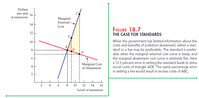
What happens if a comparable error is made in setting the standard? The efficient standard is 8 units of emissions. But suppose the standard is relaxed by 12.5 percent, from 8 to 9 units. As before, this change will lead to an increase in social costs and a decrease in abatement costs. But the net increase in social costs, given by the small triangle ADE, is much smaller than before.
This example illustrates the difference between standards and fees. When the marginal external cost curve is relatively steep and the marginal cost of abatement curve relatively flat, the cost of not reducing emissions is high. In such cases, a standard is preferable to a fee. With incomplete information, standards offer more certainty about emissions levels but leave the costs of abatement uncertain. Fees, on the other hand, offer certainty about the costs of abatement but leave the reduction of emissions levels uncertain. The preferable policy depends, therefore, on the nature of uncertainty and on the shapes of the cost curves.[2]
4. Tradeable Emissions Permits
If we knew the costs and benefits of abatement and if all firms’ costs were identical, we could apply a standard. Alternatively, if the costs of abatement varied among firms, an emissions fee would work. However, when firms’ costs vary and we do not know the costs and benefits, neither a standard nor a fee will generate an efficient outcome.
We can reach the goal of reducing emissions efficiently by using tradeable emissions permits. Under this system, each firm must have permits to generate emissions. Each permit specifies the number of units of emissions that the firm is allowed to put out. Any firm that generates emissions not allowed by permit is subject to substantial monetary sanctions. Permits are allocated among firms, with the total number of permits chosen to achieve the desired maximum level of emissions. Permits are marketable: They can be bought and sold.
Under the permit system, the firms least able to reduce emissions are those that purchase permits. Thus, suppose the two firms in Figure 18.6 (page 670) were given permits to emit up to 7 units. Firm 1, facing a relatively high marginal cost of abatement, would pay up to $3.75 to buy a permit for one unit of emissions, but the value of that permit is only $2.50 to Firm 2. Firm 2 should therefore sell its permit to Firm 1 for a price between $2.50 and $3.75.
If there are enough firms and permits, a competitive market for permits will develop. In market equilibrium, the price of a permit equals the marginal cost of abatement for all firms; otherwise, a firm will find it advantageous to buy more permits. The level of emissions chosen by the government will be achieved at minimum cost. Those firms with relatively low marginal cost of abatement curves will be reducing emissions the most, and those with relatively high marginal cost of abatement curves will be buying more permits and reducing emissions the least.
Marketable emissions permits create a market for externalities. This market approach is appealing because it combines some of the advantageous features of a system of standards with the cost advantages of a fee system. The agency that administers the system determines the total number of permits and, therefore, the total amount of emissions, just as a system of standards would do. But the marketability of the permits allows pollution abatement to be achieved at minimum cost.
Source: Pindyck Robert, Rubinfeld Daniel (2012), Microeconomics, Pearson, 8th edition.
Wow! Thank you! I always needed to write on my website something like that. Can I implement a part of your post to my site?