Bundling

You have probably seen the 1939 film Gone with the Wind. It is a classic that is nearly as popular now as it was then.13  Yet we would guess that you have not seen Getting Gertie’s Garter, a flop that the same company (MGM, a division of Loews) also distributed. And we would also guess that you did not know that these two films were priced in what was then an unusual and innovative way.14

Movie theaters that leased Gone with the Wind also had to lease Getting Gertie’s Garter. (Movie theaters pay the film companies or their distributors a daily or weekly fee for the films they lease.) In other words, these two films were bundled—i.e., sold as a package.15  Why would the film company do this?

You might think that the answer is obvious: Gone with the Wind was a great film and Gertie was a lousy film, so bundling the two forced movie theaters to lease Gertie. But this answer doesn’t make economic sense. Suppose a theater ’s reservation price (the maximum price it will pay) for Gone with the Wind is $12,000 per week, and its reservation price for Gertie is $3000 per week. Then the most it would pay for both films is $15,000, whether it takes the films individually or as a package.

Bundling makes sense when customers have heterogeneous demands and when the firm cannot price discriminate. With films, different movie theaters serve different groups of patrons and therefore different theaters may face different demands for films. For example, different theaters might appeal to different age groups, who in turn have different relative film preferences.

To see how a film company can use customer heterogeneity to its advantage, suppose that there are two movie theaters and that their reservation prices for our two films are as follows:

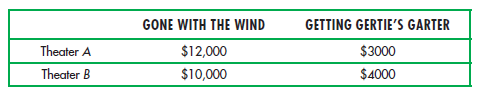
If the films are rented separately, the maximum price that could be charged for Wind is $10,000 because charging more would exclude Theater B. Similarly, the maximum price that could be charged for Gertie is $3000. Charging these two prices would yield $13,000 from each theater, for a total of $26,000 in revenue. But suppose the films are bundled. Theater A values the pair of films at $15,000 ($12,000 + $3000), and Theater B values the pair at $14,000 ($10,000 + $4000). Therefore, we can charge each theater $14,000 for the pair of films and earn a total revenue of $28,000. Clearly, we can earn more revenue ($2000 more) by bundling the films.

1. Relative Valuations

Why is bundling more profitable than selling the films separately? Because (in this example) the relative valuations of the two films are reversed. In other words, although both theaters would pay much more for Wind than for Gertie, Theater A would pay more than Theater B for Wind ($12,000 vs. $10,000), while Theater B would pay more than Theater A for Gertie ($4000 vs. $3000). In technical terms, we say that the demands are negatively correlated—the customer willing to pay the most for Wind is willing to pay the least for Gertie. To see why this is critical, suppose demands were positively correlated—that is, Theater A would pay more for both films:

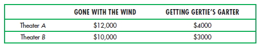
The most that Theater A would pay for the pair of films is now $16,000, but the most that Theater B would pay is only $13,000. Thus if we bundled the films, the maximum price that could be charged for the package is $13,000, yielding a total revenue of $26,000, the same as by renting the films separately.

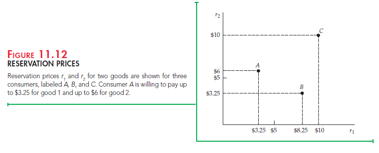
Now, suppose a firm is selling two different goods to many consumers. To analyze the possible advantages of bundling, we will use a simple diagram to describe the preferences of the consumers in terms of their reservation prices and their consumption decisions given the prices charged. In Figure 11.12 the horizontal axis is r1, which is the reservation price of a consumer for good 1, and the vertical axis is r2, which is the reservation price for good 2. The figure shows the reservation prices for three consumers. Consumer A is willing to pay up to $3.25 for good 1 and up to $6 for good 2; consumer B is willing to pay up to $8.25 for good 1 and up to $3.25 for good 2; and consumer C is willing to pay up to $10 for each of the goods. In general, the reservation prices for any number of consumers can be plotted this way.

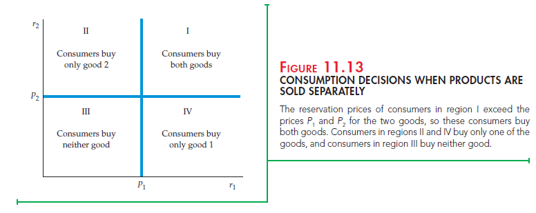
Suppose that there are many consumers and that the products are sold sepa- rately, at prices P1  and P2, respectively. Figure 11.13 shows how consumers can be divided into groups. Consumers in region I of the graph have reservation prices that are above the prices being charged for each of the goods, so they will buy both goods. Consumers in region II have a reservation price for good 2 that is above P2, but a reservation price for good 1 that is below P1; they will buy only good 2. Similarly, consumers in region IV will buy only good 1. Finally, consum- ers in region III have reservation prices below the prices charged for each of the goods, and so will buy neither.

Now suppose the goods are sold only as a bundle, for a total price of PB. We can then divide the graph into two regions, as in Figure 11.14. Any given consumer will buy the bundle only if its price is less than or equal to the sum of that consumer ’s reservation prices for the two goods. The dividing line is there- fore the equation PB = r1 + r2 or, equivalently, r2 = PB − r1. Consumers in region I have reservation prices that add up to more than PB, so they will buy the bundle. Consumers in region II, who have reservation prices that add up to less than PB, will not buy the bundle.

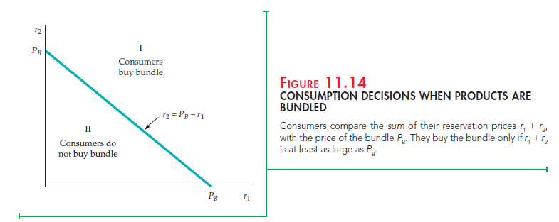
Depending on the prices, some of the consumers in region II of Figure 11.14 might have bought one of the goods if they had been sold separately. These con- sumers are lost to the firm, however, when it sells the goods only as a bundle. The firm, then, must determine whether it can do better by bundling.

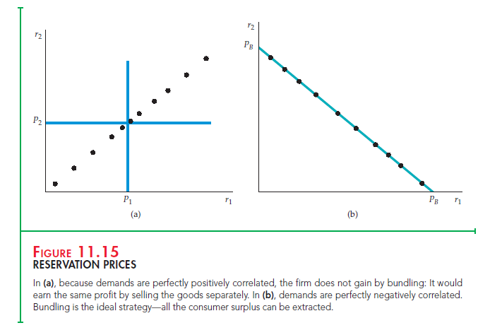
In general, the effectiveness of bundling depends on the extent to which demands are negatively correlated. In other words, it works best when consum- ers who have a high reservation price for good 1 have a low reservation price for good 2, and vice versa. Figure 11.15 shows two extremes. In part (a), each point represents the two reservation prices of a consumer. Note that the demands for the two goods are perfectly positively correlated—consumers with a high reservation price for good 1 also have a high reservation price for good 2. If the firm bundles and charges a price PB  = P1  + P2, it will make the same profit that

it would make by selling the goods separately at prices P1 and P2. In part (b), on the other hand, demands are perfectly negatively correlated—a higher reserva-tion price for good 2 implies a proportionately lower one for good 1. In this case, bundling is the ideal strategy. By charging the price PB  the firm can capture all the consumer surplus.

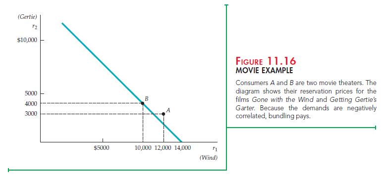
Figure 11.16, which shows the movie example that we introduced at the beginning of this section, illustrates how the demands of the two movie theaters are negatively correlated. (Theater A will pay relatively more for Gone with the Wind, but Theater B will pay relatively more for Getting Gertie’s Garter.) This makes it more profitable to rent the films as a bundle priced at $14,000.

2. Mixed Bundling

So far, we have assumed that the firm has two options: to sell the goods either separately or as a bundle. But there is a third option, called mixed bundling. As the name suggests, the firm offers its products both separately and as a bundle, with a package price below the sum of the individual prices. (We use the term pure bundling to refer to the strategy of selling the products only as a bundle.) Mixed bundling is often the ideal strategy when demands are only somewhat negatively correlated and/or  when marginal production costs are significant. (Thus far, we have assumed that marginal production costs are zero.)

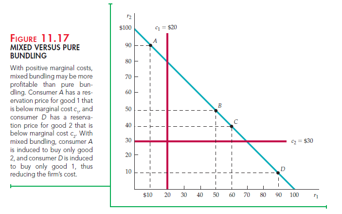
In Figure 11.17, mixed bundling is the most profitable strategy. Although demands are perfectly negatively correlated, there are significant marginal costs. (The marginal cost of producing good 1 is $20, and the marginal cost of producing good 2 is $30.) We have four consumers, labeled A through D. Now, let’s compare three strategies:

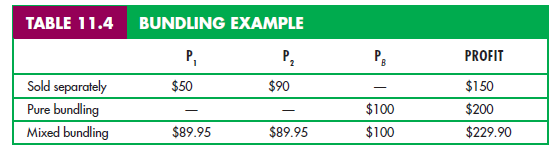
1. Selling the goods separately at prices P1 = $50 and P2 = $90
2. Selling the goods only as a bundle at a price of $100
3. Mixed bundling,  whereby  the  goods  are  offered  separately  at  prices P1 = P2 = $89.95, or as a bundle at a price of $100.

Table 11.4 shows these three strategies and the resulting profits. (You can try other prices for P1, P2, and PB  to verify that those given in the table maximize profit for each strategy.) When the goods are sold separately, only consumers B, C, and D buy good 1, and only consumer A buys good 2; total profit is 3($50 −

$20) + 1($90 − $30) = $150. With pure bundling, all four consumers buy the bundle for $100, so that total profit is 4($100 − $20 − $30) = $200. As we should expect, pure bundling is better than selling the goods separately because con- sumers’ demands are negatively correlated. But what about mixed bundling?

Consumer D buys only good 1 for $89.95, consumer A buys only good 2 for $89.95, and consumers B and C buy the bundle for $100. Total profit is now

($89.95 − $20) + ($89.95 − $30) + 2($100 − $20 − $30) = $229.90.16

In this case, mixed bundling is the most profitable strategy, even though demands are perfectly negatively correlated (i.e., all four consumers have reservation prices on the line r2  = 100 − r1). Why? For each good, marginal production cost exceeds the reservation price of one consumer. For example, consumer A has a reservation price of $90 for good 2 but a reservation price of only $10 for good 1. Because the cost of producing a unit of good 1 is $20, the firm would prefer that consumer A buy only good 2, not the bundle. It can achieve this goal by offering good 2 separately for a price just below consumer A’s reservation price, while also offering the bundle at a price acceptable to consumers B and C.

Mixed bundling would not be the preferred strategy in this example if marginal costs were zero: In that case, there would be no benefit in excluding consumer A from buying good 1 and consumer D from buying good 2. We leave it to you to demonstrate this (see Exercise 12).17

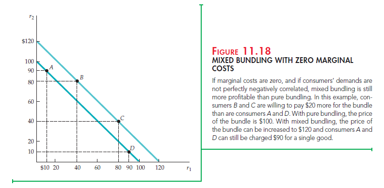
If marginal costs are zero, mixed bundling can still be more profitable than pure bundling if consumers’ demands are not perfectly negatively correlated. (Recall that in Figure 11.17, the reservation prices of the four consumers are perfectly negatively correlated.) This is illustrated by Figure 11.18, in which we have modified the example of Figure 11.17. In Figure 11.18, marginal costs are zero, but the reservation prices for consumers B and C are now higher. Once again, let’s compare three strategies: selling the two goods separately, pure bundling, and mixed bundling.

Table 11.5 shows the optimal prices and the resulting profits for each strat- egy. (Once again, you should try other prices for P1, P2, and PB  to verify that those given in the table maximize profit for each strategy.) When the goods are sold separately, only consumers C and D buy good 1, and only consum- ers A and B buy good 2; total profit is thus $320. With pure bundling, all four

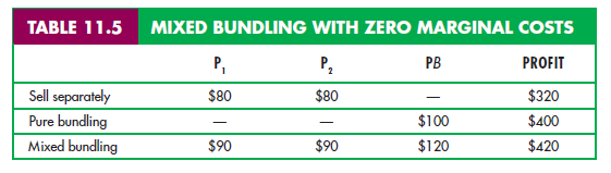
consumers buy the bundle for $100, so that total profit is $400. As expected, pure bundling is better than selling the goods separately because consumers’ demands are negatively correlated. But mixed bundling is better still. With mixed bundling, consumer A buys only good 2, consumer D buys only good

1, and consumers B and C buy the bundle at a price of $120. Total profit is now $420.

Why does mixed bundling give higher profits than pure bundling even though marginal costs are zero? The reason is that demands are not perfectly negatively correlated: The two consumers who have high demands for both goods (B and C) are willing to pay more for the bundle than are consumers A and D. With mixed bundling, therefore, we can increase the price of the bundle (from $100 to $120), sell this bundle to two consumers, and charge the remaining consumers $90 for a single good.

3. Bundling in Practice

Bundling is a widely used pricing strategy. When you buy a new car, for example, you can purchase such options as power windows, power seats, or a sunroof separately, or you can purchase a “luxury package” in which these options are bundled. Manufacturers of luxury cars (such as Lexus, BMW, or Infiniti) tend to include such “options” as standard equipment; this practice is pure bundling. For more moderately priced cars, however, these items are optional, but are usually offered as part of a bundle. Automobile companies must decide which items to include in such bundles and how to price them.

Another example is vacation travel. If you plan a vacation to Europe, you might make your own hotel reservations, buy an airplane ticket, and order a rental car. Alternatively, you might buy a vacation package in which airfare, land arrangements, hotels, and even meals are all bundled together.

Still another example is cable television. Cable operators typically offer a basic service for a low monthly fee, plus individual “premium” channels, such as Cinemax, Home Box Office, and the Disney Channel, on an individual basis for additional monthly fees. However, they also offer packages in which two or more premium channels are sold as a bundle. Bundling cable channels is profit- able because demands are negatively correlated. How do we know that? Given that there are only 24 hours in a day, the time that a consumer spends watching HBO is time that cannot be spent watching the Disney Channel. Thus consum- ers with high reservation prices for some channels will have relatively low res- ervation prices for others.

How can a company decide whether to bundle its products, and determine the profit-maximizing prices? Most companies do not know their customers’ reservation prices. However, by conducting market surveys, they may be able to estimate the distribution of reservation prices, and then use this information to design a pricing strategy.

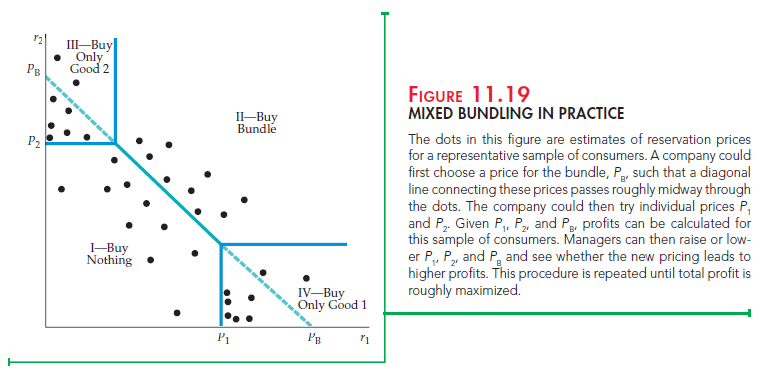
This is illustrated in Figure 11.19. The dots are estimates of reservation prices or a representative sample of consumers (obtained, say, from a market survey). The company might first choose a price for the bundle, PB, such that a diago- nal line connecting these prices passes roughly midway through the dots in the figure. It could then try individual prices P1  and P2. Given P1, P2, and PB, we can separate consumers into four regions, as shown in the figure. Consumers in Region I buy nothing (because r1 < P1, r2 < P2, and r1 + r2 < PB). Consumers in Region II buy the bundle (because r1 + r2> PB). Consumers in Region III buy only good 2 (because r2> P2  but r1  < PB  − P2). Likewise, consumers in Region IV buy only good 1. Given this distribution, we can calculate the resulting profits. We can then raise or lower P1, P2, and PB  and see whether doing so leads to higher profits. This can be done repeatedly (on a computer) until prices are found that roughly maximize total profit.

Source: Pindyck Robert, Rubinfeld Daniel (2012), Microeconomics, Pearson, 8th edition.