Externalities

Externalities can arise between producers, between customers, or between consumers and producers. They can be negative—when the action of one party imposes costs on another party—or positive—when the action of one party benefits another party.

A negative externality occurs, for example, when a steel plant dumps its waste in a river that fishermen downstream depend on for their daily catch. The more waste the steel plant dumps in the river, the fewer fish will be supported. The firm, however, has no incentive to account for the exter­nal costs that it imposes on fishermen when making its production decision. Furthermore, there is no market in which these external costs can be reflected in the price of steel. A positive externality occurs when a home owner repaints her house and plants an attractive garden. All the neighbors benefit from this activ­ity, even though the home owner’s decision to repaint and landscape probably did not take these benefits into account.

1. Negative Externalities and Inefficiency

Because externalities are not reflected in market prices, they can be a source of economic inefficiency. When firms do not take into account the harms associ­ated with negative externalities, the result is excess production and unnecessary social costs. To see why, let’s take our example of a steel plant dumping waste in a river. Figure 18.1 (a) shows the production decision of a steel plant in a com­petitive market. Figure 18.1 (b) shows the market demand and supply curves, assuming that all steel plants generate similar externalities. We assume that because the firm has a fixed-proportions production function, it cannot alter its input combinations; waste and other effluent can be reduced only by lower­ing output. (Without this assumption, firms would be jointly choosing among a variety of combinations of output and pollution abatement.) We will analyze the nature of the externality under two circumstances: first when only one steel plant pollutes and, second, when all steel plants pollute in the same way.

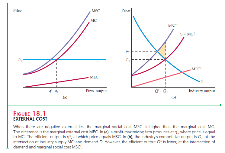
The price of steel is P₁ at the intersection of the demand and supply curves in Figure 18.1 (b). The MC curve in (a) gives a typical steel firm’s marginal cost of production. The firm maximizes profit by producing output q₁, at which marginal cost is equal to price (which equals marginal revenue because the firm takes price as given). As the firm’s output changes, however, the external cost imposed on fishermen downstream also changes. This external cost is given by the marginal external cost (MEC) curve in Figure 18.1 (a). It is intuitively clear why total external cost increases with output—there is more pollution. However, our analysis focuses on the marginal external cost, which measures the added cost of the externality associated with each additional unit of output produced. In practice, the MEC curve is upward sloping for most forms of pol­lution: As the firm produces additional output and dumps additional effluent, the incremental harm to the fishing industry increases.

From a social point of view, the firm produces too much output. The efficient level of output is the level at which the price of the product is equal to the mar­ginal social cost (MSC) of production: the marginal cost of production plus the marginal external cost of dumping effluent. In Figure 18.1 (a), the marginal social cost curve is obtained by adding marginal cost and marginal external cost for each level of output (i.e., MSC = MC + MEC). The marginal social cost curve MSC intersects the price line at output q*. Because only one plant is dumping effluent into the river, the market price of the product is unchanged. However, the firm is producing too much output (q₁ instead of q*) and generating too much effluent.

Now consider what happens when all steel plants dump their effluent into rivers. In Figure 18.1 (b), the MC¹ curve is the industry supply curve. The mar­ginal external cost associated with the industry output, MEC^I, is obtained by summing the marginal cost of every person harmed at each level of output. The MSC¹ curve represents the sum of the marginal cost of production and the mar­ginal external cost for all steel firms. As a result, MSC¹ = MC¹ + MEC¹.

Is industry output efficient when there are externalities? As Figure 18.1 (b) shows, the efficient industry output level is the level at which the mar­ginal benefit of an additional unit of output is equal to the marginal social cost. Because the demand curve measures the marginal benefit to consumers, the efficient output is Q*, at the intersection of the marginal social cost MSC^I and demand D curves. The competitive industry output, however, is at Q₁, the intersection of the demand curve and the supply curve, MC^I. Clearly, industry output is too high.

In our example, each unit of output results in some effluent being dumped. Therefore, whether we are looking at one firm’s pollution or the entire indus­try’s, the economic inefficiency is the excess production that results in too much effluent being dumped in the river. The source of the inefficiency is the incor­rect pricing of the product. The market price P₁ in Figure 18.1 (b) is too low— it reflects the firms’ marginal private cost of production, but not the marginal social cost. Only at the higher price P* will steel firms produce the efficient level of output.

What is the cost to society of this inefficiency? For each unit produced above Q*, the social cost is given by the difference between the marginal social cost and the marginal benefit (the demand curve). As a result, the aggregate social cost is shown in Figure 18.1 (b) as the shaded triangle between MSC’, D, and output Q₁. When we move from the profit-maximizing to the socially efficient output, firms are worse off because their profits are reduced, and purchasers of steel are worse off because the price of steel has increased. However, these losses are less than the gain to those who were harmed by the adverse effect of the dumping of effluent in the river.

Externalities generate both long-run and short-run inefficiencies. In Chapter 8, we saw that firms enter a competitive industry whenever the price of the product is above the average cost of production and exit whenever price is below average cost. In long-run equilibrium, price is equal to (long-run) average cost. When there are negative externalities, the average private cost of production is less than the average social cost. As a result, some firms remain in the industry even when it would be efficient for them to leave. Thus, negative externalities encourage too many firms to remain in the industry.

2. Positive Externalities and Inefficiency

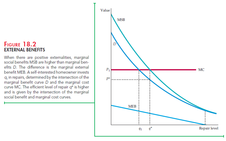
Externalities can also result in too little production, as the example of home repair and landscaping shows. In Figure 18.2, the horizontal axis measures the home owner’s investment (in dollars) in repairs and landscaping. The marginal cost curve for home repair shows the cost of repairs as more work is done on the house; it is horizontal because this cost is unaffected by the amount of repairs. The demand curve D measures the marginal private benefit of the repairs to the homeowner. The home owner will choose to invest q in repairs, at the intersec­tion of her demand and marginal cost curves. But repairs generate external ben­efits to the neighbors, as the marginal external benefit curve, MEB, shows. This curve is downward sloping in this example because the marginal benefit is large for a small amount of repair but falls as the repair work becomes extensive.

The marginal social benefit curve, MSB, is calculated by adding the marginal private benefit and the marginal external benefit at every level of output. In short, MSB = D + MEB. The efficient level of output q*, at which the marginal social benefit of additional repairs is equal to the marginal cost of those repairs, is found at the intersection of the MSB and MC curves. The inefficiency arises because the homeowner doesn’t receive all the benefits of her investment in repairs and landscaping. As a result, the price P₁ is too high to encourage her to invest in the socially desirable level of house repair. A lower price, P*, is required to encourage the efficient level of supply, q*.

Another example of a positive externality is the money that firms spend on research and development (R&D). Often the innovations resulting from research cannot be protected from other firms. Suppose, for example, that a firm designs a new product. If that design can be patented, the firm might earn a large profit by manufacturing and marketing the product. But if the new design can be closely imitated by other firms, those firms can appropriate some of the developing firm’s profit. Because there is then little reward for doing R&D, the market is likely to underfund it.

The externality concept is not new: In discussing demand in Chapter 4, we explained that positive and negative network externalities can arise if the quan­tity of a good demanded by a consumer increases or decreases in response to an increase in purchases by other consumers. Network externalities can also lead to market failures. Suppose, for example, that some individuals enjoy socializing at busy ski resorts when many other skiers are present. The resulting conges­tion could make the skiing experience unpleasant for those skiers who preferred short lift lines to pleasant social occasions.

Source: Pindyck Robert, Rubinfeld Daniel (2012), Microeconomics, Pearson, 8th edition.