In panel data, the rationale behind random effects model is that: unlike the fixed-effects model, the variation across entities is assumed to be random and uncorrelated with the independent variables included in the model. So, “…the crucial distinction between fixed and random effects is whether the unobserved individual effect embodies elements that are correlated with the regressors in the model, not whether these effects are stochastic or not” (Green, 2008, p.183).
Random effects assume that the entity’s error term is not correlated with the independent variables which allow for time-invariant variables to play a role as independent variables.
If we have reason to believe that differences across entities have some influence on our dependent variable, then we should use random effects. An advantage of random effects is that: we can include time invariant variables (such as superficies of province). In the fixed effects model, these variables are absorbed by the intercept.
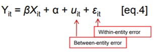
The random effects model is:
Random effects assume that the entity’s error term is not correlated with the predictors which allows for time-invariant variables to play a role as explanatory variables.
In random-effects, we need to specify those individual characteristics that may or may not influence the independent variables. The problem with this is that some variables may not be available therefore leading to omitted variable bias in the model.
RE allows to generalize the inferences beyond the sample used in the model.
Our panel data used in the video, that you can download here in Stata datasheet or Excel data, includes 434 year-observations of 62 provinces as entities of our sample; each province has 7 year-observations. These data were collected from the statistical yearbooks of Vietnam’s provinces during the period from 2010 to 2016; then cleaned by eliminating some missing-data provinces and year-observations.
The Stata command to run fixed/random effects is xtreg.
Before using xtreg you need to set Stata to handle panel data by using the command xtset. Type: xtset Id Year, yearly. Note that Stata distinguishes capital letters, so you must type exactly the variable name. Or you can click this command on the Stata’s Menu by avoiding typing errors.
In this case, “Id” represents the entities that is Vietnam provinces; and “Year” represents the time variable t.
As the panel data has been handled, we can now run the random-effects model by using the Stata command xtreg with the same variables by choosing the option re, for dependent variable ANS and 13 variables, including 11 independent ones and 2 control variables.
Type: xtreg ANS FDIENT FDICAP FDIAST FDIEMP FDICOM FDIWAG FDITUR FDIGDP FDIROTC FDIROFA FDIROS Size GDPgrowth, re.
Or you can click this command on the Stata’s Menu by avoiding typing errors.

I genuinely enjoy looking through on this web site, it has good content.
Very well written post. It will be valuable to anyone who utilizes it, as well as myself. Keep doing what you are doing – for sure i will check out more posts.
You have brought up a very fantastic details , thanks for the post.