Coefficient of Determination

For the Armand’s Pizza Parlors example, we developed the estimated regression equation y = 60 + 5x to approximate the linear relationship between the size of the student popu­lation x and quarterly sales y. A question now is: How well does the estimated regression equation fit the data? In this section, we show that the coefficient of determination pro­vides a measure of the goodness of fit for the estimated regression equation.

For the ith observation, the difference between the observed value of the dependent variable, y_t, and the predicted value of the dependent variable, y, is called the ith residual. The ith residual represents the error in using y, to estimate y. Thus, for the ith observation, the residual is y_i – y,. The sum of squares of these residuals or errors is the quantity that is minimized by the least squares method. This quantity, also known as the sum of squares due to error, is denoted by SSE.

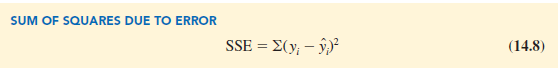
The value of SSE is a measure of the error in using the estimated regression equation to predict the values of the dependent variable in the sample.

In Table 14.3 we show the calculations required to compute the sum of squares due to error for the Armand’s Pizza Parlors example. For instance, for restaurant 1 the values of the independent and dependent variables are x₁ = 2 and y₁ = 58. Using the estimated regression equation, we find that the predicted value of quarterly sales for restaurant 1 is y₁ = 60 + 5(2) = 70. Thus, the error in using y₁ to predict y₁ for restaurant 1 is y₁ – y₁ = 58 – 70 = -12. The squared error, (—12)² = 144, is shown in the last column of Table 14.3. After computing and squaring the residuals for each restaurant in the sample, we sum them to obtain SSE = 1530. Thus, SSE = 1530 measures the error in using the estimated regression equation y = 60 + 5x to predict sales.

Now suppose we are asked to develop an estimate of quarterly sales without knowledge of the size of the student population. Without knowledge of any related variables, we would use the sample mean as an estimate of quarterly sales at any given restaurant.

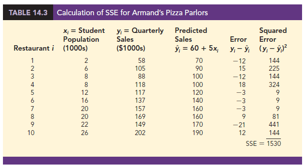
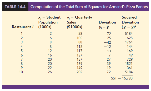
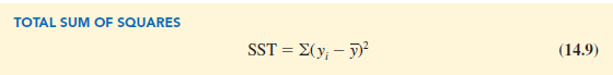
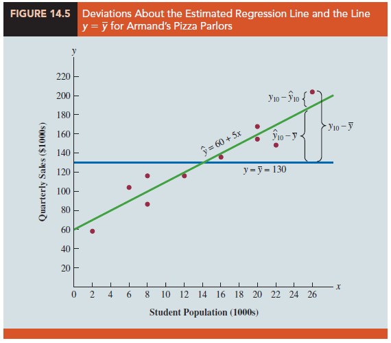
Table 14.2 showed that for the sales data, oyi = 1300. Hence, the mean value of quarterly sales for the sample of 10 Armand’s restaurants is y = oyi/n = 1300/10 = 130. In Table 14.4 we show the sum of squared deviations obtained by using the sample mean y = 130 to predict the value of quarterly sales for each restaurant in the sample. For the ith restaurant in the sample, the difference yi − y provides a measure of the error involved in using y to predict sales. The corresponding sum of squares, called the total sum of squares, is denoted SST.

The sum at the bottom of the last column in Table 14.4 is the total sum of squares for Armand’s Pizza Parlors; it is SST = 15,730.

In Figure 14.5 we show the estimated regression line y = 60 + 5x and the line cor­responding to y = 130. Note that the points cluster more closely around the estimated regression line than they do about the line y = 130. For example, for the 10th restaurant in the sample we see that the error is much larger when y = 130 is used to predict y₁₀ than when y₁₀ = 60 + 5(26) = 190 is used. We can think of SST as a measure of how well the observations cluster about the y line and SSE as a measure of how well the observations cluster about the y line.

To measure how much the y values on the estimated regression line deviate from y, another sum of squares is computed. This sum of squares, called the sum of squares due to regression, is denoted SSR.

From the preceding discussion, we should expect that SST, SSR, and SSE are related. Indeed, the relationship among these three sums of squares provides one of the most im­portant results in statistics.

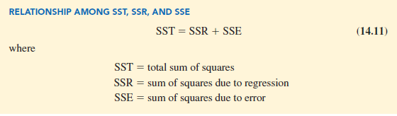
Equation (14.11) shows that the total sum of squares can be partitioned into two compon­ents, the sum of squares due to regression and the sum of squares due to error. Hence, if the values of any two of these sum of squares are known, the third sum of squares can be computed easily. For instance, in the Armand’s Pizza Parlors example, we already know that SSE = 1530 and SST = 15,730; therefore, solving for SSR in equation (14.11), we find that the sum of squares due to regression is

SSR = SST – SSE = 15,730 – 1530 = 14,200

Now let us see how the three sums of squares, SST, SSR, and SSE, can be used to provide a measure of the goodness of fit for the estimated regression equation. The estimated regression equation would provide a perfect fit if every value of the dependent variable y happened to lie on the estimated regression line. In this case, y – y would be zero for each observation, resulting in SSE = 0. Because SST = SSR + SSE, we see that for a perfect fit SSR must equal SST, and the ratio (SSR/SST) must equal one. Poorer fits will result in larger values for SSE. Solving for SSE in equation (14.11), we see that SSE = SST – SSR. Hence, the largest value for SSE (and hence the poorest fit) occurs when SSR = 0 and SSE = SST.

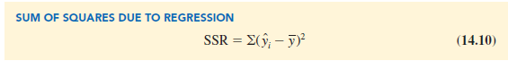
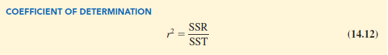
The ratio SSR/SST, which will take values between zero and one, is used to evaluate the goodness of fit for the estimated regression equation. This ratio is called the coefficient of determination and is denoted by r².

For the Armand’s Pizza Parlors example, the value of the coefficient of determination is

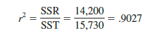
When we express the coefficient of determination as a percentage, r² can be interpreted as the percentage of the total sum of squares that can be explained by using the estimated regression equation. For Armand’s Pizza Parlors, we can conclude that 90.27% of the total sum of squares can be explained by using the estimated regression equation y = 60 + 5x to predict quarterly sales. In other words, 90.27% of the variability in sales can be explained by the linear relationship between the size of the student population and sales. We should be pleased to find such a good fit for the estimated regression equation.

Correlation Coefficient

In Chapter 3 we introduced the correlation coefficient as a descriptive measure of the strength of linear association between two variables, x and y. Values of the correlation coefficient are always between – 1 and + 1. A value of + 1 indicates that the two variables x and y are perfectly related in a positive linear sense. That is, all data points are on a straight line that has a positive slope. A value of – 1 indicates that x and y are perfectly related in a negative linear sense, with all data points on a straight line that has a negative slope. Values of the correlation coefficient close to zero indicate that x and y are not linearly related.

In Section 3.5 we presented the equation for computing the sample correlation coeffi­cient. If a regression analysis has already been performed and the coefficient of determina­tion r² computed, the sample correlation coefficient can be computed as follows:

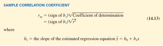
The sign for the sample correlation coefficient is positive if the estimated regression equa­tion has a positive slope (b₁ > 0) and negative if the estimated regression equation has a negative slope (b₁ < 0).

For the Armand’s Pizza Parlor example, the value of the coefficient of determina­tion corresponding to the estimated regression equation y = 60 + 5x is .9027. Because the slope of the estimated regression equation is positive, equation (14.13) shows that the sample correlation coefficient is + √.9027 = + .9501. With a sample correlation coefficient of ^rxy = + .9501, we would conclude that a strong positive linear association exists between x and y.

In the case of a linear relationship between two variables, both the coefficient of determination and the sample correlation coefficient provide measures of the strength of the relationship. The coefficient of determination provides a measure between zero and one, whereas the sample correlation coefficient provides a measure between -1 and +1. Although the sample correlation coefficient is restricted to a linear relationship between two variables, the coefficient of determination can be used for nonlinear relationships and for relationships that have two or more independent variables. Thus, the coefficient of determination provides a wider range of applicability.

Source:  Anderson David R., Sweeney Dennis J., Williams Thomas A. (2019), Statistics for Business & Economics, Cengage Learning; 14th edition.