Data processing in quantitative studies

1. Editing

Irrespective of the method of data collection, the information collected is called raw data or simply data. The first step in processing your data is to ensure that the data is ‘clean’ — that is, free from inconsistencies and incompleteness. This process of ‘cleaning’ is called editing.

Editing consists of scrutinising the completed research instruments to identify and mini­mise, as far as possible, errors, incompleteness, misclassification and gaps in the information obtained from the respondents. Sometimes even the best investigators can:

• forget to ask a question;
• forget to record a response;
• wrongly classify a response;
• write only half a response;
• write illegibly.

In the case of a questionnaire, similar problems can crop up. These problems to a great extent can be reduced simply by (1) checking the contents for completeness, and (2) checking the responses for internal consistency.

The way you check the contents for completeness depends upon the way the data has been collected. In the case of an interview, just checking the interview schedule for the above problems may improve the quality of the data. It is good practice for an interviewer to take a few moments to peruse responses for possible incompleteness and inconsistencies. In the case of a questionnaire, again, just by carefully checking the responses some of the problems may be reduced. There are several ways of minimising such problems:

• By inference – Certain questions in a research instrument may be related to one another and it might be possible to find out the answer to one question from the answer to another. Of course, you must be careful about making such inferences or you may introduce new errors into the data.
• By recall – if the data is collected by means of interviews, sometimes it might be possible for the interviewer to recall a respondent’s answers. Again, you must be extremely careful.
• By going back to the respondent – if the data has been collected by means of interviews or the questionnaires contain some identifying information, it is possible to visit or phone a respond­ent to confirm or ascertain an answer. This is, of course, expensive and time consuming.

There are two ways of editing the data:

• examine all the answers to one question or variable at a time;
• examine all the responses given to all the questions by one respondent at a time.

The author prefers the second method as it provides a total picture of the responses, which also helps you to assess their internal consistency.

2. Coding

Having ‘cleaned’ the data, the next step is to code it. The method of coding is largely dictated by two considerations:

1. the way a variable has been measured (measurement scale) in your research instrument (e.g. if a response to a question is descriptive, categorical or quantitative);
2. the way you want to communicate the findings about a variable to your readers.

For coding, the first level of distinction is whether a set of data is qualitative or quantitative in nature. For qualitative data a further distinction is whether the information is descriptive in nature (e.g. a description of a service to a community, a case history) or is generated through discrete qualitative categories. For example, the following information about a respondent is in discrete qualitative categories: income — above average, average, below average; gender — male, female; religion — Christian, Hindu, Muslim, Buddhist, etc.; or attitude towards an issue — strongly favourable, favourable, uncertain, unfavourable, strongly unfavourable. Each of these variables is measured either on a nominal scale or an ordinal scale. Some of them could also have been measured on a ratio scale or an interval scale. For example, income can be measured in dollars (ratio scale), or an attitude towards an issue can be measured on an interval or a ratio scale. The way you proceed with the coding depends upon the measurement scale used in the measurement of a variable and whether a question is open-ended or closed.

In addition, the types of statistical procedures that can be applied to a set of information to a large extent depend upon the measurement scale on which a variable was measured in the research instrument. For example, you can find out different statistical descriptors such as mean, mode and median if income is measured on a ratio scale, but not if it is measured on an ordinal or a nominal scale. It is extremely important to understand that the way you are able to analyse a set of information is dependent upon the measurement scale used in the research instrument for measuring a variable. It is therefore important to visualise — particularly at the planning stage when constructing the research instrument — the way you are going to com­municate your findings.

How you can analyse information obtained in response to a question depends upon how a question was asked, and how a respondent answered it. In other words, it depends upon the measurement scale on which a response can be measured/classified. If you study answers given by your respondents in reply to a question, you will realise that almost all responses can be classified into one of the following three categories:

1. quantitative responses;
2. categorical responses (which may be quantitative or qualitative);
3. descriptive responses (which are invariably qualitative – keep in mind that this is qualitative data collected as part of quantitative research and not the qualitative research).

For the purpose of analysis, quantitative and categorical responses need to be dealt with differently from descriptive ones. Both quantitative and categorical information go through a process that is primarily aimed at transforming the information into numerical values, called codes, so that the information can be easily analysed, either manually or by computers. On the other hand, descriptive information first goes through a process called content analysis, whereby you identify the main themes that emerge from the descriptions given by respondents in answer to questions. Having identified the main themes, there are three ways that you can deal with them: (1) you can examine verbatim responses and integrate them with the text of your report to either support or contradict your argument; (2) you can assign a code to each theme and count how frequently each has occurred; and (3) you can combine both methods to communicate your findings. This is your choice, and it is based on your impression of the preference of your readers.

For coding quantitative and qualitative data in quantitative studies you need to go through the following steps:

• Step I developing a code book;
• Step II pre-testing the code book;
• Step III coding the data;
• Step IV verifying the coded data.

Step I: Developing a code book

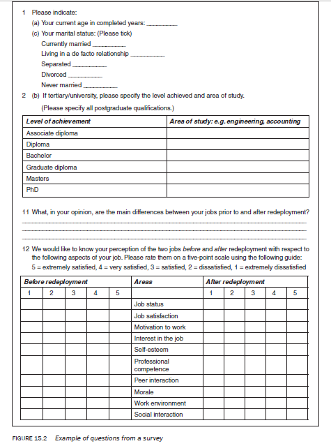
A code book provides a set of rules for assigning numerical values to answers obtained from respondents. Let us take an example. Figure 15.2 lists some questions taken from a question­naire used in a survey conducted by the author to ascertain the impact of occupational rede­ployment on an individual. The questions selected should be sufficient to serve as a prototype for developing a code book, as they cover the various issues involved in the process.

There are two formats for data entry: ‘fixed’ and ‘free’. In this chapter we will be using the fixed format to illustrate how to develop a code book. The fixed format stipulates that a piece of information obtained from a respondent is entered in a specific column. Each column has a number and the ‘Col. no.’ in the code book refers to the column in which a specific type of information is to be entered. The information about an individual is thus entered in a row(s) comprising these columns.

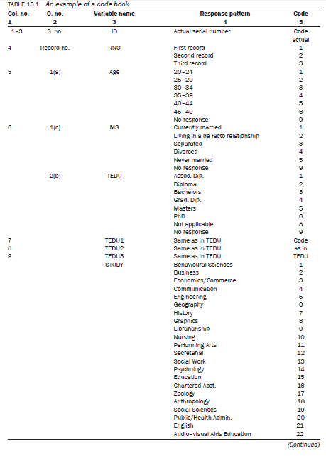
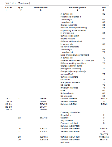
For a beginner it is important to understand the structure of a code book (Table 15.1), which is based on the responses given to the questions listed in Figure 15.2.

In Table 15.1, column 1 refers to the columns in which a particular piece of information is to be entered. Allocation of columns in a fixed format is extremely important because, when you write a program, you need to specify the column in which a particular piece of information is entered so that the computer can perform the required procedures.

Column 2 identifies the question number in the research instrument for which the infor­mation is being coded. This is primarily to identify coding with the question number in the instrument.

Column 3 refers to the name of the variable. Each variable in a program is given a unique name so that the program can carry out the requested statistical procedures. Usually there are restrictions on the way you can name a variable (e.g. the number of characters you can use to name a variable and whether you use the alphabet or numerals). You need to check your program for this. It is advisable to name a variable in such a way that you can easily recognise it from its name.

Column 4 lists the responses to the various questions. Developing a response pattern for the questions is the most important, difficult and time-consuming part of developing a code book. The degree of difficulty in developing a response pattern differs with the types of ques­tions in your research instrument (open ended or closed). If a question is closed, the response pattern has already been developed as part of the instrument construction and all you need to do at this stage is to assign a numerical value to each response category. In terms of analysis, this is one of the main advantages of closed questions. If a closed question includes ‘other’ as one of the response categories, to accommodate any response that you may not have listed when developing the instrument, you should analyse the responses and assign them to non­overlapping categories in the same way as you would do for open-ended questions. Add these to the already developed response categories and assign each a numerical value.

If the number of responses to a question is less than nine, you need only one column to code the responses, and if it is more than nine but less than 99, you need two columns (col­umn 1 in the code book). But if a question asks respondents to give more than one response, the number of columns assigned should be in accordance with the number of responses to be coded. If there are, say, eight possible responses to a particular question and a respondent is asked to give three responses, you need three columns to code the responses to the question. Let us assume there are 12 possible responses to a question. To code each response you need two columns and, therefore, to code three responses you need six columns.

The coding of open-ended questions is more difficult. Coding of open-ended questions requires the response categories to be developed first through a process called content analysis. One of the easier ways of analysing open-ended questions is to select a number of inter­view schedules/questionnaires randomly from the total completed interview schedules or questionnaires received. Then select an open-ended question from one of these schedules or questionnaires and write down the response(s) on a sheet of paper. If the person has given more than one response, write them separately on the same sheet. Similarly, from the same questionnaire/schedule select another open-ended question and write down the responses given on a separate sheet. In the same way you can select other open-ended questions and write down the response(s). Remember that the response to each question should be written on a separate sheet. Now select another questionnaire/interview schedule and go through the same process, adding response(s) given for the same question on the sheet for that question. Continue the process until you feel that the responses are being repeated and you are getting no or very few new ones — that is, when you have reached a saturation point.

Now, one by one, examine the responses to each question to ascertain the similarities and differences. If two or more responses are similar in meaning though not necessarily in lan­guage, try to combine them under one category. Give a name to the category that is descrip­tive of the responses. Remember, when you code the data you code categories, not responses per se. It is advisable to write down the different responses under each category in the code book so that, while coding, you know the type of responses you have grouped under a cat­egory. In developing these categories there are three important considerations:

1. The categories should be mutually Develop non-overlapping categories. A response should not be able to be placed within two categories.
2. The categories should be exhaustive; that is, almost every response should be able to be placed within one of the categories. If too many responses cannot be so categorised, it is an indication of ineffective categorisation. in such a situation you should examine your categories again.
3. The use of the ‘other category, effectively a ‘waste basket’ for those odd responses that cannot be put into any category, must be kept to the absolute minimum because, as mentioned, it reflects the failure of the classification system. This category should not include more than 5 per cent of the total responses and should not contain any more responses than any other category.

Column 5 lists the actual codes of the code book that you decide to assign to a response. You can assign any numerical value to any response so long as you do not repeat it for another response within the same question. Two responses to questions are commonly repeated: ‘not applicable’ and ‘no response’. You should select a number that can be used for these responses for all or most questions. For example, responses such as ‘not applicable’ and ‘no response’ could be given a code of 8 and 9 respectively, even though the responses to a question may be limited to only 2 or 3. In other words, suppose you want to code the gender of a respondent and you have decided to code female = 1 and male = 2. For ‘no response’, instead of assigning a code of 3, assign a code of 9. This suggestion helps in remembering codes, which will help to increase your speed in coding.

To explain how to code, let us take the questions listed in the example in Figure 15.2. We will take each question one by one to detail the process.

Question 1(a)

Your current age in completed years: ______

This is an open-ended quantitative question. In questions like this it is important to determine the range of responses — the respondent with the lowest and the respondent with the highest age. To do this, go through a number of questionnaires/interview schedules. Once the range is established, divide it into a number of categories. The categories developed are dependent upon a number of considerations such as the purpose of analysis, the way you want to com­municate the findings of your study and whether the findings are going to be compared with those of another study. Let us assume that the range in the study is 23 to 49 years and assume that you develop the following categories to suit your purpose: 20—24, 25—29, 30—34, 35—39, 40—44 and 45—49. If your range is correct you should need no other categories. Let us assume that you decide to code 20—24 = 1,25—29 = 2, 30—34 = 3, and so on. To accommodate ‘no response’ you decide to assign a code of 9. Let us assume you decided to code the responses to this question in column 5 of the code sheet.

Question 1(c)

Your marital status: (Please tick)

Currently married______

Living in a de facto relationship_

Separated___________

Divorced____________

Never married________

This is a closed categorical question. That is, the response pattern is already provided. In these situations you just need to assign a numerical value to each category. For example, you may decide to code ‘currently married’ = 1, ‘living in a de facto relationship’ = 2, ‘separated’ = 3, ‘divorced’ = 4 and ‘never married’ = 5. You may add ‘no response’ as another category and assign it with a code of 9. The response to this question is coded in column 6 of the code sheet.

Question 2(b)

If tertiary/university, please specify the level achieved and the area of study. (Please specify all postgradu­ate qualifications.)

In this question a respondent is asked to indicate the area in which s/he has achieved a terti­ary qualification. The question asks for two aspects: (1) level of achievement, which is cat­egorical; and (2) area of study, which is open ended. Also, a person may have more than one qualification which makes it a multiple response question. In such questions both aspects of the question are to be coded. In this case, this means the level of achievement (e.g. associate diploma, diploma) and the area of study (e.g. engineering, accounting). When coding multiple responses, decide on the maximum possible number of responses to be coded. Let us assume you code a maximum number of three levels of tertiary education. (This would depend upon the maximum number of levels of achievement identified by the study population.) Firstly, code the levels of achievement tedu (tedu: t = tertiary and edu = education; the naming of

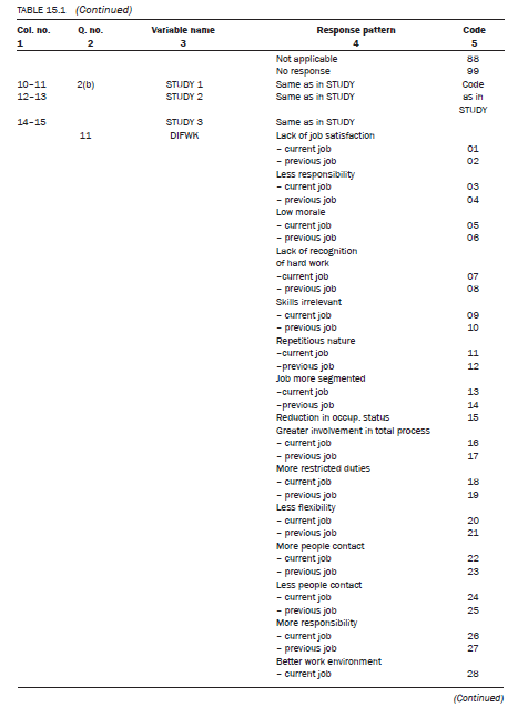
the variable — ‘level of achievement’ — in this manner is done for easy identification) and then the area of study, study (the variable name given to the ‘area of study’ = study) . In the above example, let us assume that you decided to code three levels of achievement. To distinguish them from each other we call the first level teduI, the second tedu2 and the third tedu3, and decide to code them in columns, 7, 8 and 9 respectively. Similarly, the names given to the three areas of study are studyI, study2 and study3 and we decide to code them in columns 10—11, 12—13 and 14—15. The codes (01 to 23) assigned to different qualifications are listed in the code book. If a respondent has only one qualification, the question of second and third qualification is not applicable and you need to decide a code for ‘not applicable’. Assume you assigned a code of 88. ‘No response’ would then be assigned a code of 99 for this question.

Question 11

What, in your opinion, are the main differences between your jobs prior to and after redeployment?

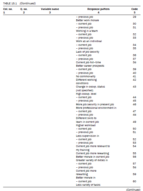
This is an open-ended question. To code this you need to go through the process of content analysis as explained earlier. Within the scope of this chapter it is not possible to explain the details, but response categories that have been listed are based upon the responses given by 109 respondents to the survey on occupational redeployment. In coding questions like this, on the one hand you need to keep the variation in the respondents’ answers and, on the other, you want to break them up into meaningful categories to identify the commonalities. Because this question is asking respondents to identify the differences between their jobs before and after redeployment, for easy identification let us assume this variable was named difwk (dif = dif­ference and wk = work). Responses to this question are listed in Figure 15.3. These responses have been selected at random from the questionnaires returned.

A close examination of these responses reveals that a number of themes are common, for example: ‘learning new skills in the new job’; ‘challenging tasks are missing from the new posi­tion’; ‘more secure in the present job’; ‘more interaction in the present job’; ‘less responsibility’; ‘more variety’; ‘no difference’; ‘more satisfying’. There are many similar themes that hold for both the before and after jobs. Therefore, we developed these themes for ‘current job’ and ‘previous job’.

One of the main differences between qualitative and quantitative research is the way responses are used in the report. In qualitative research the responses are normally used either verbatim or are organised under certain themes and the actual responses are provided to sub­stantiate them.

In quantitative research the responses are examined, common themes are identified, the themes are named (or categories are developed) and the responses given by respondents are classified under these themes. The data then can also be analysed to determine the frequency of the themes if so desired. It is also possible to analyse the themes in relation to some other characteristics such as age, education and income of the study population.

The code book lists the themes developed on the basis of responses given. As you can see, many categories may result. The author’s advice is not to worry about this as categories can always be combined later if required. The reverse is impossible unless you go back to the raw data.

Let us assume you want to code up to five responses to this question and that you have decided to name these five variables as difwkI, difwk2, difwk3, difwk4 and difwk5. Let us also assume that you have coded them in columns 16—17, 18—19, 20—21, 22—23 and 24—25 respectively.

Question 12

We would like to know your level of satisfaction with the two jobs before and after redeploy­ment with respect to the following aspects of your job. Please rate them on a five-point scale using the following guide:

5 = extremely satisfied, 4 = very satisfied, 3 = satisfied, 2 = dissatisfied, 1 = extremely dissatisfied

This is a highly structured question asking respondents to compare on a five-point ordinal scale their level of satisfaction with various areas of their job before and after redeployment. As we are gauging the level of satisfaction before and after redeployment, respondents are expected to give two responses to each area. In this example let us assume you have used the name jobsta for job status after redeployment (job = job, st = status and a = after redeployment) and jobstb for before redeployment (job = job, st = status and b = before redeployment). Similarly, for the second area, job satisfaction, you have decided that the variable name, jobsata (job = job, sat = satisfaction and a = after), will stand for the level of job satisfaction after redeployment and jobsatb will stand for the level before redeployment. Other variable names have been similarly assigned. In this example the variable, jobsta, is entered in column 26, jobstb in column 27, and so on.

Step II: Pre-testing the code book

Once a code book is designed, it is important to pre-test it for any problems before you code your data. A pre-test involves selecting a few questionnaires/interview schedules and actually coding the responses to ascertain any problems in coding. It is possible that you may not have provided for some responses and therefore will be unable to code them. Change your code book, if you need to, in light of the pre-test.

Step III: Coding the data

Once your code book is finalised, the next step is to code the raw data. There are three ways of doing this:

1. coding on the questionnaires/interview schedule itself, if space for coding was provided at the time of constructing the research instrument;
2. coding on separate code sheets that are available for purchase;
3. coding directly into the computer using a program such as sPssx, sAs.

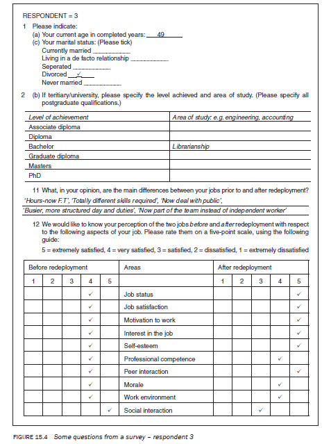
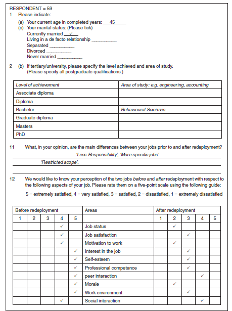
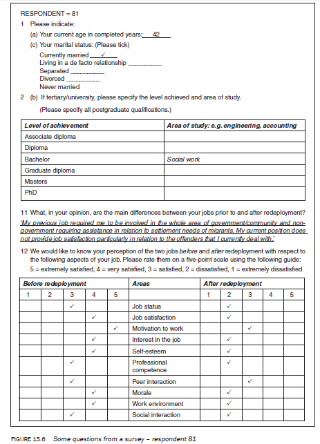
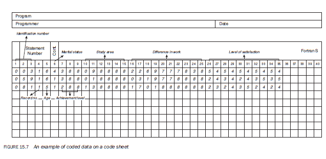
To explain the process of coding let us take the same questions that were used in develop­ing the code book. We select three questionnaires at random from a total of 109 respondents (Figures 15.4, 15.5, 15.6). Using the code book as a guide, we code the information from these sheets onto the coding sheet (Figure 15.7). Let us examine the coding process by taking respondent 3 (Figure 15.4).

Respondent 3

The total number of respondents is more than 99 and this is the third questionnaire, so 003 was given as the identification number which is coded in columns 1—3 (Figure 15.7). Because it is the first record for this respondent, 1 was coded in column 4. This respondent is 49 years of age and falls in the category 45—49, which was coded as 6. As the information on age is entered in column 5, 6 was coded in this column of the code sheet. The marital status of this person is ‘divorced’, hence 4 was coded in column 6. This person has a Bachelors degree in librarianship. The code chosen for a Bachelors degree is 3, which was entered in column 7. Three tertiary qualifications have been provided for, and as this person does not have any other qualifications, tedu2 and tedu3 are not applicable, and therefore a code of 8 is entered in columns 8 and 9. This person’s Bachelors degree is in librarianship for which code 09 was assigned and entered in columns 10—11. Since there is only one qualification, study2 and study3 are not applicable; therefore, a code of 88 was entered in columns 12—13 and 14—15. This person has given a number of responses to question no. 11 (difwk), which asks respondents to list the main differences between their jobs before and after redeployment. In coding such questions much caution is required.

Examine the responses named difwkI, difwk2, difwk3, difwk4 and difwk5, to identify the codes that can be assigned. A code of 22 (now deal with public) was assigned to one of the responses, which we enter in columns 16—17. The second difference, difwk2, was assigned a code of 69 (totally different skill required), which is coded in columns 18—19.

difwk3 was assigned a code of 77 (current job more structure) and coded in columns 20—21. Similarly, the fourth (difwk4) and the fifth (difwk5) difference in the jobs before and after redeployment are coded as 78 (now part of the team instead of independent worker) and 38 (hours — now full time), which are entered in columns 22—23 and 24—25 respectively. Question 12 is extremely simple to code. Each area of a job has two columns, one for before and the other for after. Job status (jobst) is divided into two variables, job- Sta for a respondent’s level of satisfaction after redeployment and jobstb for his/her level before redeployment. jobsta is entered in column 26 and jobstb in column 27. For jobsta the code, 5 (as marked by the respondent), is entered in column 26 and the code for job­stb, 4, is entered in column 27. Other areas of the job before and after redeployment are similarly coded.

The other two examples are coded in the same manner. The coded data is shown in Figure 15.7. In the process of coding you might find some responses that do not fit your predetermined categories. If so, assign them a code and add these to your code book.

Step IV: Verifying the coded data

Once the data is coded, select a few research instruments at random and record the responses to identify any discrepancies in coding. Continue to verify coding until you are sure that there are no discrepancies. If there are discrepancies, re-examine the coding.

Developing a frame of analysis

Although a framework of analysis needs to evolve continuously while writing your report, it is desirable to broadly develop it before analysing the data. A frame of analysis should specify:

• which variables you are planning to analyse;
• how they should be analysed;
• what cross-tabulations you need to work out;
• which variables you need to combine to construct your major concepts or to develop indices (in formulating a research problem concepts are changed to variables – at this stage change them back to concepts);
• which variables are to be subjected to which statistical procedures.

To illustrate, let us take the example from the survey used in this chapter.

Frequency distributions

A frequency distribution groups respondents into the subcategories into which a vari­able can be divided. Unless you are not planning to use answers to some of the questions, you should have a frequency distribution for all the variables. Each variable can be specified either separately or collectively in the frame of analysis. To illustrate, they are identified here separately by the names used in the code book. For example, frame of analysis should include frequency distribution for the following variables:

• age;
• ms;
• tedu (teduI, tedu2, tedu3 – multiple responses, to be collectively analysed);
• study (studyI, study2, study3 – multiple responses, to be collectively analysed);
• difwk (difwkI, difwk2, difwk3, difwk4, difwk5 – multiple responses, to be collectively analysed);
• jobsta, jobstb;
• jobsata, jobsatb;
• motiva, motivb.

Cross-tabulations

Cross-tabulations analyse two variables, usually independent and dependent or attribute and dependent, to determine if there is a relationship between them. The subcategories of both the variables are cross-tabulated to ascertain if a relationship exists between them. Usually, the absolute number of respondents, and the row and column percentages, give you a reasonably good idea as to the possible association.

In the study we cited as an example in this chapter, one of the main variables to be explained is the level of satisfaction with the ‘before’ and ‘after’ jobs after redeployment. We developed two indices of satisfaction:

1. satisfaction with the job before redeployment (satindb);
2. satisfaction with the job after redeployment (satinda).

Differences in the level of satisfaction can be affected by a number of personal attributes such as the age, education, training and marital status of the respondents. Cross-tabulations help to identify which attributes affect the levels of satisfaction. Theoretically, it is possible to correlate any variables, but it is advisable to be selective or an enormous number of tables will result. Normally only those variables that you think have an effect on the dependent variable should be correlated. The following cross-tabulations are an example of the basis of a frame of analysis.You can specify as many variables as you want. satinda and satindb by:

• age;
• ms;
• tedu;
• study;
• difwk.

These determine whether job satisfaction before and after redeployment is affected by age, marital status, education, and so on.

• satinda by satindb.
• This ascertains whether there is a relationship between job satisfaction before and after redeployment.

Reconstructing the main concepts

There may be places in a research instrument where you look for answers through a number of questions about different aspects of the same issue, for example the level of satisfaction with jobs before and after redeployment (satindb and satinda). In the questionnaire there were 10 aspects of a job about which respondents were asked to identify their level of satisfaction before and after redeployment. The level of satisfaction may vary from aspect to aspect. Though it is important to know respondents’ reactions to each aspect, it is equally important to gauge an overall index of their satisfaction. You must therefore ascertain, before you actually analyse data, how you will combine responses to different questions.

In this example the respondents indicated their level of satisfaction by selecting one of the five response categories. A satisfaction index was developed by assigning a numerical value — the greater the magnitude of the response category, the higher the numerical score — to the response given by a respondent. The numerical value corresponding to the category ticked was added to determine the satisfaction index. The satisfaction index score for a respondent varies between 10 and 50. The interpretation of the score is dependent upon the way the numerical values are assigned. In this example the higher the score, the higher the level of satisfaction.

Statistical procedures

In this section you should list the statistical procedures that you want to subject your data to. You should identify the procedures followed by the list of variables that will be subjected to those procedures. For example,

Regression analysis:

• satinda and satindb

Multiple regression analysis:

• satinda with age, education, ms.
• satindb with age, education, ms.

Analysis of variance (anova):

Similarly, it may be necessary to think about and specify the different variables to be sub­jected to the various statistical procedures. There are a number of user-friendly programs such as SPSSx and SAS that you can easily learn.

Analysing quantitative data manually

Coded data can be analysed manually or with the help of a computer. If the number of respondents is reasonably small, there are not many variables to analyse, and you are neither familiar with a relevant computer program nor wish to learn one, you can manually analyse the data. However, manual analysis is useful only for calculating frequencies and for simple cross-tabulations. If you have not entered data into a computer but want to carry out statisti­cal tests, they will have to be calculated manually, which may become extremely difficult and time consuming. However, the use of statistics depends upon your expertise and desire/need to communicate the findings in a certain way.

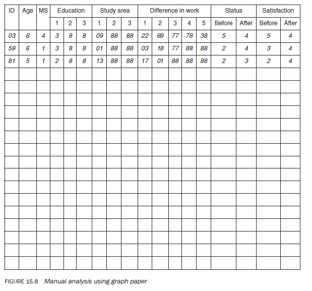
Be aware that manual analysis is extremely time consuming. The easiest way to analyse data manually is to code it directly onto large graph paper in columns in the same way as you would enter it into a computer. On the graph paper you do not need to worry about the column number. Detailed headings can be used or question numbers can be written on each column to code information about the question (Figure 15.8).

To analyse data manually (frequency distributions), count various codes in a column and then decode them. For example, age from Figure 15.8, 5 = 1, 6 = 2. This shows that out of the three respondents, one was between 40 and 44 years of age and the other two were between 45 and 49. Similarly, responses for each variable can be analysed. For cross­tabulations two columns must be read simultaneously to analyse responses in relation to each other.

If you want to analyse data using a computer, you should be familiar with the appropriate program. You should know how to create a data file, how to use the procedures involved, what statistical tests to apply and how to interpret them. Obviously in this area knowledge of computers and statistics plays an important role.

Source: Kumar Ranjit (2012), Research methodology: a step-by-step guide for beginners, SAGE Publications Ltd; Third edition.