Once we define the decision alternatives and the states of nature for the chance events, we can focus on determining probabilities for the states of nature. The classical method, the relative frequency method, or the subjective method of assigning probabilities may be used to identify these probabilities. After determining the appropriate probabilities, we show how to use the expected value approach to identify the best, or recommended, decision alternative for the problem.
1. Expected Value Approach
We begin by defining the expected value of a decision alternative. Let
N = the number of states of nature
P(Sj) = the probability of state of nature Sj
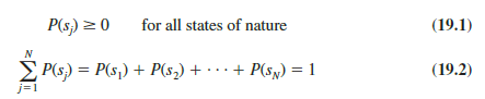
Because one and only one of the N states of nature can occur, the probabilities must satisfy two conditions:
The expected value (EV) of decision alternative dt is as follows:

In words, the expected value of a decision alternative is the sum of weighted payoffs for the decision alternative. The weight for a payoff is the probability of the associated state of nature and therefore the probability that the payoff will occur. Let us return to the PDC problem to see how the expected value approach can be applied.
PDC is optimistic about the potential for the luxury high-rise condominium complex. Suppose that this optimism leads to an initial subjective probability assessment of .8 that demand will be strong (s1) and a corresponding probability of .2 that demand will be weak (s2). Thus, P(s1) = .8 and P(s2) = .2. Using the payoff values in Table 19.1 and equation (19.3) , we compute the expected value for each of the three decision alternatives as follows:
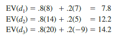
Thus, using the expected value approach, we find that the large condominium complex, with an expected value of $14.2 million, is the recommended decision.
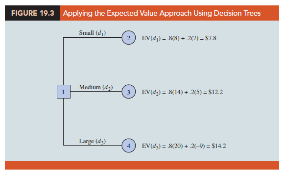
The calculations required to identify the decision alternative with the best expected value can be conveniently carried out on a decision tree. Figure 19.2 shows the decision tree for the PDC problem with state-of-nature branch probabilities. Working backward through the decision tree, we first compute the expected value at each chance node; that is, at each chance node, we weight each possible payoff by its probability of occurrence. By doing so, we obtain the expected values for nodes 2, 3, and 4, as shown in Figure 19.3.
Because the decision maker controls the branch leaving decision node 1 and because we are trying to maximize the expected profit, the best decision alternative at node 1 is d3. Thus, the decision tree analysis leads to a recommendation of d3 with an expected value of $14.2 million. Note that this recommendation is also obtained with the expected value approach in conjunction with the payoff table.
Other decision problems may be substantially more complex than the PDC problem, but if a reasonable number of decision alternatives and states of nature are present, you can use the decision tree approach outlined here. First, draw a decision tree consisting of decision nodes, chance nodes, and branches that describe the sequential nature of the problem. If you use the expected value approach, the next step is to determine the probabilities for each of the states of nature and compute the expected value at each chance node. Then select the decision branch leading to the chance node with the best expected value. The decision alternative associated with this branch is the recommended decision.

2. Expected Value of Perfect Information
Suppose that PDC has the opportunity to conduct a market research study that would help evaluate buyer interest in the condominium project and provide information that management could use to improve the probability assessments for the states of nature. To determine the potential value of this information, we begin by supposing that the study could provide perfect information regarding the states of nature; that is, we assume for the moment that PDC could determine with certainty, prior to making a decision, which state of nature is going to occur. To make use of this perfect information, we will develop a decision strategy that PDC should follow once it knows which state of nature will occur. A decision strategy is simply a decision rule that specifies the decision alternative to be selected after new information becomes available.
To help determine the decision strategy for PDC, we reproduce PDC’s payoff table in Table 19.2. Note that, if PDC knew for sure that state of nature s1 would occur, the best decision alternative would be d3, with a payoff of $20 million. Similarly, if PDC knew for sure that state of nature s2 would occur, the best decision alternative would be d1, with a payoff of $7 million. Thus, we can state PDC’s optimal decision strategy if the perfect information becomes available as follows:
If s1, select d3 and receive a payoff of $20 million.
If s2, select d1 and receive a payoff of $7 million.

What is the expected value for this decision strategy? To compute the expected value with perfect information, we return to the original probabilities for the states of nature: P(s1) = .8 and P(s2) = .2. Thus, there is a .8 probability that the perfect information will indicate state of nature s1 and the resulting decision alternative d3 will provide a $20 million profit. Similarly, with a .2 probability for state of nature s2, the optimal decision alternative d1 will provide a $7 million profit. Thus, using equation (19.3), the expected value of the decision strategy based on perfect information is
.8(20) + .2(7) = 17.4
We refer to the expected value of $17.4 million as the expected value with perfect information (EVwPI).
Earlier in this section we showed that the recommended decision using the expected value approach is decision alternative d3, with an expected value of $14.2 million. Because this decision recommendation and expected value computation were made without the benefit of perfect information, $14.2 million is referred to as the expected value without perfect information (EVwoPI).
The expected value with perfect information is $17.4 million, and the expected value without perfect information is $14.2; therefore, the expected value of the perfect information (EVPI) is $17.4 — $14.2 = $3.2 million. In other words, $3.2 million represents the additional expected value that can be obtained if perfect information were available about the states of nature. Generally speaking, a market research study will not provide “perfect” information; however, if the market research study is a good one, the information gathered might be worth a sizable portion of the $3.2 million. Given the EVPI of $3.2 million, PDC might seriously consider a market survey as a way to obtain more information about the states of nature.
In general, the expected value of perfect information (EVPI) is computed as follows:
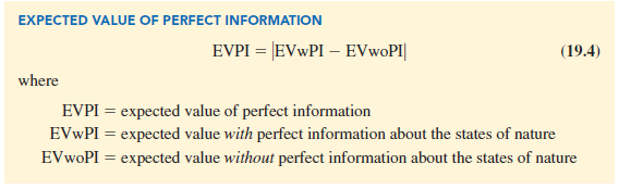
Note the role of the absolute value in equation (19.4). For minimization problems, information helps reduce or lower cost; thus the expected value with perfect information is less than or equal to the expected value without perfect information. In this case, EVPI is the magnitude of the difference between EVwPI and EVwoPI, or the absolute value of the difference as shown in equation (19.4).
Source: Anderson David R., Sweeney Dennis J., Williams Thomas A. (2019), Statistics for Business & Economics, Cengage Learning; 14th edition.
28 Aug 2021
30 Aug 2021
28 Aug 2021
31 Aug 2021
28 Aug 2021
30 Aug 2021