In Chapter 2, we encountered some simplified versions of the basic present value formula. Let us see whether they offer any insights into stock values. Suppose, for example, that we forecast a constant growth rate for a company’s dividends. This does not preclude year-to-year deviations from the forecast: It means only that expected dividends grow at a constant rate. Such an investment would be just another example of the growing perpetuity that we valued in Chapter 2. To find its present value we must divide the first year’s cash payment by the difference between the discount rate and the growth rate:
![]()
Remember that we can use this formula only when g, the anticipated growth rate, is less than r, the discount rate. As g approaches r, the stock price becomes infinite. Obviously, r must be greater than g if growth really is perpetual.
Our growing perpetuity formula explains P0 in terms of next year’s expected dividend DIV1, the projected growth trend g, and the expected rate of return on other securities of comparable risk r. Alternatively, the formula can be turned around to obtain an estimate of r from DIV1, P0, and g:
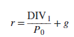
The expected return equals the dividend yield (DIV1/P0) plus the expected rate of growth in dividends (g).
These two formulas are much easier to work with than the general statement that “price equals the present value of expected future dividends.”[1] Here is a practical example.
1. Using the DCF Model to Set Water, Gas, and Electricity Prices
In the United States, the prices charged by local water, electric, and gas utilities are regulated by state commissions. The regulators try to keep consumer prices down but are supposed to allow the utilities to earn a fair rate of return. But what is fair? It is usually interpreted as r, the market capitalization rate for the firm’s common stock. In other words, the fair rate of return on equity for a public utility ought to be the cost of equity—that is, the rate offered by securities that have the same risk as the utility’s common stock.[2]
Small variations in estimates of this return can have large effects on the prices charged to the customers and on the firm’s profits. So both the firms’ managers and regulators work hard to estimate the cost of equity. They’ve noticed that most utilities are mature, stable companies that pay regular dividends. Such companies should be tailor-made for application of the constant-growth DCF formula.
Suppose you wished to estimate the cost of equity for Aqua America, a local water distribution company. Aqua’s stock (ticker symbol WTR) was selling for $33.62 per share at the end of September 2017. Dividend payments for the next year were expected to be $1.18 a share. Thus, it was a simple matter to calculate the first half of the DCF formula:
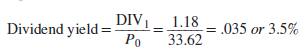
The hard part is estimating g, the expected rate of dividend growth. One option is to consult the views of security analysts who study the prospects for each company. Analysts are rarely prepared to stick their necks out by forecasting dividends to kingdom come, but they often forecast growth rates over the next five years, and these estimates may provide an indication of the expected long-run growth path. In the case of Aqua, analysts in 2017 were forecasting an annual growth of 6.6%.[3] This, together with the dividend yield, gave an estimate of the cost of equity capital:
![]()
An alternative approach to estimating long-run growth starts with the payout ratio, the ratio of dividends to earnings per share (EPS). For Aqua, this ratio has averaged about 60%. In other words, each year the company was plowing back into the business about 40% of earnings per share:
![]()
Also, Aqua’s ratio of earnings per share to book equity per share has averaged about 12.6%. This is its return on equity, or ROE:
![]()
If Aqua earns 12.6% on book equity and reinvests 40% of earnings, then book equity will increase by .40 X .126 = .05, or 5%. Earnings and dividends per share will also increase by 5%:
![]()
That gives a second estimate of the market capitalization rate:
![]()
Although these estimates of Aqua’s cost of equity seem reasonable, there are obvious dangers in analyzing any single firm’s stock with the constant-growth DCF formula. First, the underlying assumption of regular future growth is at best an approximation. Second, even if it is an acceptable approximation, errors inevitably creep into the estimate of g.
Remember, Aqua’s cost of equity is not its personal property. In well-functioning capital markets, investors capitalize the dividends of all securities in Aqua’s risk class at exactly the same rate. But any estimate of r for a single common stock is “noisy” and subject to error. Good practice does not put too much weight on single-company estimates of the cost of equity. It collects samples of similar companies, estimates r for each, and takes an average. The average gives a more reliable benchmark for decision making.
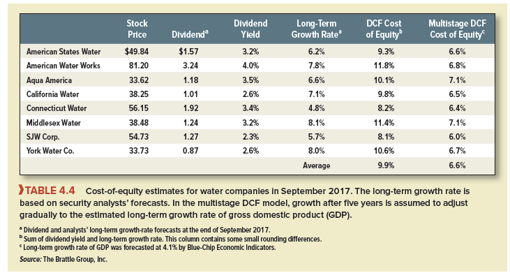
The next-to-last column of Table 4.4 gives DCF cost-of-equity estimates for Aqua and seven other water companies. These are all stable, mature companies for which the constant-growth DCF formula ought to work. Notice the variation in the cost-of-equity estimates. Some of the variation may reflect differences in the risk, but some is just noise. The average estimate is 9.9%.
Estimates of this kind are only as good as the long-term forecasts on which they are based. For example, several studies have observed that security analysts are subject to behavioral biases and their forecasts tend to be overoptimistic. If so, such DCF estimates of the cost of equity should be regarded as upper estimates of the true figure.
2. Dangers Lurk in Constant-Growth Formulas
The simple constant-growth DCF formula is an extremely useful rule of thumb, but no more than that. Naive trust in the formula has led many financial analysts to silly conclusions.
We have stressed the difficulty of estimating r by analysis of one stock only. Try to use a large sample of equivalent-risk securities. Even that may not work, but at least it gives the analyst a fighting chance because the inevitable errors in estimating r for a single security tend to balance out across a broad sample.
Also, resist the temptation to apply the formula to firms having high current rates of growth. Such growth can rarely be sustained indefinitely, but the constant-growth DCF formula assumes it can. This erroneous assumption leads to an overestimate of r.
Example The U.S. Surface Transportation Board (STB) tracks the “revenue adequacy” of U.S. railroads by comparing the railroads’ returns on book equity with estimates of their costs of equity. To estimate the cost of equity, the STB traditionally used the constant-growth formula. It measured g by stock analysts’ forecasts of long-term earnings growth. The formula assumes that earnings and dividends grow at a constant rate forever, but the analysts’ “longterm” forecasts looked out five years at most. As the railroads’ profitability improved, the analysts became more and more optimistic. By 2009, their forecasts for growth averaged 12.5% per year. The average dividend yield was 2.6%, so the constant-growth model estimated the industry-average cost of capital at 2.6 + 12.5 = 15.1%.
So the STB said, in effect, “Wait a minute: Railroad earnings and dividends can’t grow at 12.5% forever. The constant-growth formula no longer works for railroads. We’ve got to find a more accurate method.” The STB now uses a multistage growth model.[4] Let us look at an example of such a model.
DCF Models with Two or More Stages of Growth Consider Growth-Tech Inc., a firm with DIVj = $.50 and P0 = $50. The firm has plowed back 80% of earnings and has had a return on equity (ROE) of 25%. This means that in the past
Dividend growth rate = plowback ratio X ROE = .80 X .25 = .20
The temptation is to assume that the future long-term growth rate g also equals .20. This would imply
![]()
But this is silly. No firm can continue growing at 20% per year forever, except possibly under extreme inflationary conditions. Eventually, profitability will fall and the firm will respond by investing less.
In real life, the return on equity will decline gradually over time, but for simplicity, let’s assume it suddenly drops to 16% at year 3 and the firm responds by plowing back only 50% of earnings. Then g drops to .50 X .16 = .08.
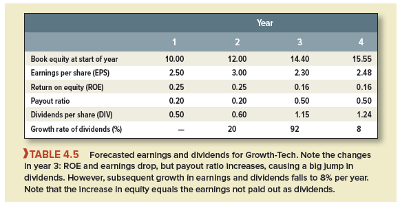
Table 4.5 shows what’s going on. Growth-Tech starts year 1 with book equity of $10.00 per share. It earns $2.50, pays out 50 cents as dividends, and plows back $2. Thus, it starts year 2 with book equity of $10 + 2 = $12. After another year at the same ROE and payout, it starts year 3 with equity of $14.40. However, ROE drops to .16, and the firm earns only $2.30. Dividends go up to $1.15 because the payout ratio increases, but the firm has only $1.15 to plow back. Therefore, subsequent growth in earnings and dividends drops to 8%.
Now we can use our general DCF formula:
![]()
Investors in year 3 will view Growth-Tech as offering 8% per year dividend growth. So we can use the constant-growth formula to calculate P3:
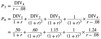
We have to use trial and error to find the value of r that makes P0 equal $50. It turns out that the r implicit in these more realistic forecasts is just over .099, quite a difference from our “constant-growth” estimate of .21.
Our present value calculations for Growth-Tech used a two-stage DCF valuation model. In the first stage (years 1 and 2), Growth-Tech is highly profitable (ROE = 25%), and it plows back 80% of earnings. Book equity, earnings, and dividends increase by 20% per year. In the second stage, starting in year 3, profitability and plowback decline, and earnings settle into long-term growth at 8%. Dividends jump up to $1.15 in year 3, and then also grow at 8%.
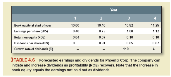
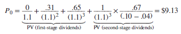
Growth rates can vary for many reasons. Sometimes, growth is high in the short run not because the firm is unusually profitable, but because it is recovering from an episode of low profitability. Table 4.6 displays projected earnings and dividends for Phoenix Corp., which is gradually regaining financial health after a near meltdown. The company’s equity is growing at a moderate 4%. ROE in year 1 is only 4%, however, so Phoenix has to reinvest all its earnings, leaving no cash for dividends. As profitability increases in years 2 and 3, an increasing dividend can be paid. Finally, starting in year 4, Phoenix settles into steady-state growth, with equity, earnings, and dividends all increasing at 4% per year.
Assume the cost of equity is 10%. Then Phoenix shares should be worth $9.13 per share:
You could go on to valuation models with three or more stages. For example, the far right column of Table 4.4 presents multistage DCF estimates of the cost of equity for our local water companies. In this case the long-term growth rates reported in the table do not continue forever. After five years, each company’s growth rate gradually adjusts down to an estimated long-term 4.1% growth rate for gross domestic product (GDP). The reduced growth rate cuts the average cost of equity to 6.6%.
We must leave you with two more warnings about DCF formulas for valuing common stocks or estimating the cost of equity. First, it’s almost always worthwhile to lay out a simple spreadsheet, like Table 4.5 or 4.6, to ensure that your dividend projections are consistent with the company’s earnings and required investments. Second, be careful about using DCF valuation formulas to test whether the market is correct in its assessment of a stock’s value. If your estimate of the value is different from the market value, it is probably because you have used poor dividend forecasts. Remember what we said at the beginning of this chapter about simple ways of making money on the stock market: There aren’t any.
Good day! This is kind of off topic but I need some guidance from an established blog. Is it tough to set up your own blog? I’m not very techincal but I can figure things out pretty fast. I’m thinking about creating my own but I’m not sure where to begin. Do you have any points or suggestions? Thanks