The Black-Scholes Formula for Valuing Options

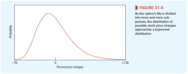
Look back at Figure 21.1, which showed what happens to the distribution of possible Amazon stock price changes as we divide the option’s life into a larger and larger number of increas­ingly small subperiods. You can see that the distribution of price changes becomes increas­ingly smooth.

If we continued to chop up the option’s life in this way, we would eventually reach the situation shown in Figure 21.4, where there is a continuum of possible stock price changes at maturity. Figure 21.4 is an example of a lognormal distribution. The lognormal distribution is often used to summarize the probability of different stock price changes.^[1] It has a number of good commonsense features. For example, it recognizes the fact that the stock price can never fall by more than 100% but that there is some, perhaps small, chance that it could rise by much more than 100%.

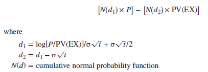
Subdividing the option life into indefinitely small slices does not affect the principle of option valuation. We could still replicate the call option by a levered investment in the stock, but we would need to adjust the degree of leverage continuously as time went by. Calculating option value when there is an infinite number of subperiods may sound a hopeless task. Fortunately, Black and Scholes derived a formula that does the trick.^[2] It is an unpleasant-looking formula, but on closer acquaintance you will find it exceptionally elegant and useful. The formula is

Notice that the value of the call in the Black-Scholes formula has the same properties that we identified earlier. It increases with the level of the stock price P and decreases with the present value of the exercise price PV(EX), which in turn depends on the interest rate and time to maturity. It also increases with the time to maturity and the stock’s variability (o Vt).

To derive their formula, Black and Scholes assumed that there is a continuum of stock prices, and therefore to replicate an option, investors must continuously adjust their holding in the stock.^[4] Of course, this is not literally possible, but even so, the formula performs remark­ably well in the real world, where stocks trade only intermittently and prices jump from one level to another. The Black-Scholes model has also proved very flexible; it can be adapted to value options on a variety of assets such as foreign currencies, bonds, and commodities. It is not surprising, therefore, that it has been extremely influential and has become the standard model for valuing options. Every day, dealers on the options exchanges use this formula to make huge trades. These dealers are not for the most part trained in the formula’s mathematical derivation; they just use a computer or a specially programmed calculator to find the value of the option.

1. Using the Black-Scholes Formula

The Black-Scholes formula may look difficult, but it is very straightforward to apply. Let us practice using it to value the Amazon call.

Here are the data that you need:

• Price of stock now = P = 900
• Exercise price = EX = 900
• Standard deviation of continuously compounded annual returns = a = .25784
• Years to maturity = t = .5
• Interest rate per annum = rf = .5% for 6 months or about 1% per annum

Remember that the Black-Scholes formula for the value of a call is

There are three steps to using the formula to value the Amazon call:

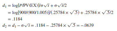
Step 1 Calculate d₁ and d₂. This is just a matter of plugging numbers into the formula (noting that “log” means natural log):

Step 2 Find N(d₁) and N(d₂). N(d₁) is the probability that a normally distributed variable will be less than d₁ standard deviations above the mean. If d₁ is large, N(d₁) is close to 1.0 (i.e., you can be almost certain that the variable will be less than d₁ standard deviations above the mean). If d₁ is zero, N(d₁) is .5 (i.e., there is a 50% chance that a normally distributed vari­able will be below the average).

The simplest way to find N(d₁) is to use the Excel function NORMSDIST. For example, if you enter NORMSDIST(.1184) into an Excel spreadsheet, you will see that there is a .5471 probability that a normally distributed variable will be less than .1184 standard deviations above the mean.

Again you can use the Excel function to find N(d₂). If you enter NORMSDIST (-.0639) into an Excel spreadsheet, you should get the answer .4745. In other words, there is a prob­ability of .4745 that a normally distributed variable will be less than .0639 standard deviations below the mean.

Step 3 Plug these numbers into the Black-Scholes formula. You can now calculate the value of the Amazon call:

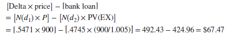
In other words, you can replicate the Amazon call option by investing $492.43 in the compa­ny’s stock and borrowing $424.96. Subsequently, as time passes and the stock price changes, you may need to borrow a little more to invest in the stock or you may need to sell some of your stock to reduce your borrowing.

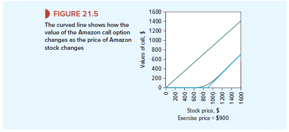
Some More Practice Suppose you repeat the calculations for the Amazon call for a wide range of stock prices. The result is shown in Figure 21.5. You can see that the option values lie along an upward-sloping curve that starts its travels in the bottom left-hand corner of the diagram. As the stock price increases, the option value rises and gradually becomes parallel to the lower bound for the option value. This is exactly the shape we deduced in Chapter 20 (see Figure 20.9).

The height of this curve of course depends on risk and time to maturity. For example, if the risk of Amazon stock had suddenly increased, the curve shown in Figure 21.5 would rise at every possible stock price. For example, Figure 20.11 shows what would happen to the curve if the risk of Amazon stock doubled.

2. The Risk of an Option

How risky is the Amazon call option? We have seen that you can exactly replicate a call by a combination of risk-free borrowing and an investment in the stock. So the risk of the option must be the same as the risk of this replicating portfolio. We know that the beta of any portfo­lio is simply a weighted average of the betas of the separate holdings. So the risk of the option is just a weighted average of the betas of the investments in the loan and the stock.

On past evidence, the beta of Amazon stock is p_stock = 1.5; the beta of a risk-free loan is p_loan = 0. You are investing $492.43 in the stock and -$424.96 in the loan. (Notice that the investment in the loan is negative—you are borrowing money.) Therefore the beta of the option is p_option = (-424.96 x 0 + 492.43 x 1.5)/(-424.96 + 492.43) = 10.95. Notice that because a call option is equivalent to a levered position in the stock, it is always riskier than the stock itself. In Amazon’s case, the option is about 7 times as risky as the stock and 11 times as risky as the market. As time passes and the price of Amazon stock changes, the risk of the option will also change.

3. The Black-Scholes Formula and the Binomial Method

Look back at Table 21.1, where we used the binomial method to calculate the value of the Amazon call. Notice that, as the number of intervals is increased, the values that you obtain from the binomial method begin to snuggle up to the Black-Scholes value of $67.47.

The Black-Scholes formula recognizes a continuum of possible outcomes. This is usually more realistic than the limited number of outcomes assumed in the binomial method. The formula is also more accurate and quicker to use than the binomial method. So why use the binomial method at all? The answer is that there are many circumstances in which you cannot use the Black-Scholes formula, but the binomial method will still give you a good measure of the option’s value. We will look at several such cases in Section 21-5.

Source:  Brealey Richard A., Myers Stewart C., Allen Franklin (2020), Principles of Corporate Finance, McGraw-Hill Education; 13th edition.