Finding the value of the stock of Boeing or GE may sound like a simple problem. Public companies publish quarterly and annual balance sheets, which list the value of the company’s assets and liabilities. For example, at the end of September 2017, the book value of all GE’s assets—plant and machinery, inventories of materials, cash in the bank, and so on—was $378 billion. GE’s liabilities—money that it owes the banks, taxes that are due to be paid, and the like—amounted to $298.5 billion. The difference between the value of the assets and the liabilities was just over $79.5 billion. This was the book value of GE’s equity.[1]
Book value is a reassuringly definite number. Each year KPMG, one of America’s largest accounting firms, gives its opinion that GE’s financial statements present fairly in all material respects the company’s financial position, in conformity with U.S. generally accepted accounting principles (commonly called GAAP). However, the book value of GE’s assets measures only their original (or “historical”) cost less an allowance for depreciation. This may not be a good guide to what those assets are worth today.
One can go on and on about the deficiencies of book value as a measure of market value. Book values are historical costs that do not incorporate inflation. (Countries with high or volatile inflation often require inflation-adjusted book values, however.) Book values usually exclude intangible assets such as trademarks and patents. Also accountants simply add up the book values of individual assets, and thus do not capture going-concern value. Going-concern value is created when a collection of assets is organized into a healthy operating business.
Book values can nevertheless be a useful benchmark. Suppose, for example, that the aggregate value of all of Holstein Oil’s shares is $900 million. Its book value of equity is $450 million. A financial analyst might say, “Holstein sells for two times book value. It has doubled shareholders’ cumulative past investment in the company.” She might also say, “Holstein’s market value added is $900 – 450 = $450 million. (There is more on market value added in Chapter 28.)
Book values may also be useful clues about liquidation value. Liquidation value is what investors get when a failed company is shut down and its assets are sold off. Book values of “hard” assets like land, buildings, vehicles, and machinery can indicate possible liquidation values.
Intangible “soft” assets can be important even in liquidation, however. Eastman Kodak provides a good example. Kodak, which was one of the Nifty Fifty growth stocks of the 1960s, suffered a long decline and finally filed for bankruptcy in January 2012. What was one of its most valuable assets in bankruptcy? Its portfolio of 79,000 patents, which was subsequently sold for $525 million.
1. Valuation by Comparables
When financial analysts need to value a business, they often start by identifying a sample of similar firms as potential comparables. They then examine how much investors in the comparable companies are prepared to pay per dollar of earnings or book assets. They see what the business would be worth if it traded at the comparables’ price-earnings or price-to-book- value ratios. This valuation approach is called valuation by comparables.
Table 4.2 tries out this valuation method for three companies and industries. Let’s start with Union Pacific (UNP). In November 2017, UNP’s stock was trading around $117. Security analysts were forecasting earnings per share (EPS) for 2018 at $6.55, giving a “forward” price-earnings ratio of P/E = 17.85.[2] UNP’s market-book ratio (price divided by book value per share) was P/B = 4.73.
P/Es and P/Bs for several of UNP’s competitors are reported on the right-hand side of the table. Notice that UNP’s P/E is close to the P/Es of these comparables. If you didn’t know UNP’s stock price, you could get an estimate by multiplying UNP’s forecasted EPS of $6.55 by 17.49, the average P/E for the comparables. The resulting estimate of $114.56 would be almost spot on. On the other hand, UNP’s P/B is higher than all the comparables’ P/Bs except for that of Canadian Pacific. If you had used the average price-to-book ratio for the comparables to value UNP, you would have come up with an underestimate of UNP’s actual share price.
Look now at Johnson & Johnson (J&J) and its four comparables in Table 4.2. In this case, the P/B ratio for J&J is higher than for the comparables (5.2 versus an average of 4.1). The average P/E for J&J is also higher (17.8 versus 15.5). An estimate of the value of J&J based on the comparables’ P/Es and P/Bs would be too low. Comparing the estimate to J&J’s actual stock price could still be worthwhile, however, if it leads you to ask why J&J was more attractive to investors.
The ratios for Devon Energy in Table 4.2 illustrate the potential difficulties with valuation by comparables. There is a huge variation in the P/E ratios of the comparables. Anadarko and Marathon had negative P/E ratios; their stock prices were of course positive, but their operations had been battered by a sudden fall in oil prices, and their forecasted earnings for the next year were negative. The average P/E of -.58 for the comparables is meaningless.[3] The comparables’ average P/B is more informative.
The P/E ratios for the oil companies in Table 4.2 illustrate what can go wrong with the ratios in hard times when firms makes losses. P/E ratios are also almost useless as a guide to the value of new start-ups, most of which do not have any earnings to compare.
Such difficulties do not invalidate the use of comparables to value businesses. Maybe Table 4.2 doesn’t show the companies most closely similar to Devon. A financial manager or analyst would need to dig deeper to understand Devon’s industry and its competitors. Also, the method might work better with different ratios.[4]
Of course, investors did not need valuation by comparables to value Devon Energy or the other companies in Table 4.2. They are all public companies with actively traded shares. But you may find valuation by comparables useful when you don’t have a stock price. For example, in August 2017 the mining giant, BHP Billiton, announced plans to sell its U.S. shale business. Preliminary estimates put the business’s value at $8 to $10 billion. It’s a safe bet that BHP and its advisers were burning the midnight oil and doing their best to identify the best comparables and check what the assets would be worth if they traded at the comparables’ P/E and P/B ratios.
But BHP would need to be cautious. As Table 4.2 shows, these ratios can vary widely even within the same industry. To understand why this is so, we need to look more carefully at what determines a stock’s market value. We start by connecting stock prices to the cash flows that stockholders receive from the company in the form of cash dividends. This will lead us to a discounted-cash-flow (DCF) model of stock prices.
2. Stock Prices and Dividends
Not all companies pay dividends. Rapidly growing companies typically reinvest earnings instead of paying out cash. But most mature, profitable companies do pay regular cash dividends.
Think back to Chapter 3, where we explained how bonds are valued. The market value of a bond equals the discounted present value (PV) of the cash flows (interest and principal payments) that the bond will pay out over its lifetime. Let’s import and apply this idea to common stocks. The future cash flows to the owner of a share of common stock are the future dividends per share that the company will pay out. Thus, the logic of discounted cash flow suggests
PV(share of stock) = PV(expected future dividends per share)
At first glance, this statement may seem surprising. Investors hope for capital gains as well as dividends. That is, they hope to sell stocks for more than they paid for them. Why doesn’t the PV of a stock depend on capital gains? As we now explain, there is no inconsistency.
Today’s Price If you own a share of common stock, your cash payoff comes in two forms: (1) cash dividends and (2) capital gains or losses. Suppose that the current price of a share is P0, that the expected price at the end of a year is P1, and that the expected dividend per share is DIV1. The rate of return that investors expect from this share over the next year is defined as the expected dividend per share DIV1 plus the expected price appreciation per share P1 – P0, all divided by the price at the start of the year P0:
![]()
Suppose Fledgling Electronics stock is selling for $100 a share (P0 = 100). Investors expect a $5 cash dividend over the next year (DIV1 = 5). They also expect the stock to sell for $110 a year, hence (P1 = 110). Then the expected return to the stockholders is 15%:
![]()
On the other hand, if you are given investors’ forecasts of dividend and price and the expected return offered by other equally risky stocks, you can predict today’s price:
![]()
For Fledgling Electronics, DIV1 = 5 and P1 = 110. If r, the expected return for Fledgling is 15%, then today’s price should be $100:
![]()
What exactly is the discount rate, r, in this calculation? It’s called the market capitalization rate or cost of equity capital, which are just alternative names for the opportunity cost of capital, defined as the expected return on other securities with the same risks as Fledgling shares.
Many stocks will be safer than Fledgling and many riskier. But among the thousands of traded stocks, there will be a group with essentially the same risks. Call this group Fledgling’s risk class. Then all stocks in this risk class have to be priced to offer the same expected rate of return.
Let’s suppose that the other securities in Fledgling’s risk class all offer the same 15% expected return. Then $100 per share has to be the right price for Fledgling stock. In fact, it is the only possible price. What if Fledgling’s price were above P0 = $100? In this case, the expected return would be less than 15%. Investors would shift their capital to the other securities and, in the process, would force down the price of Fledgling stock. If P0 were less than $100, the process would reverse. Investors would rush to buy, forcing the price up to $100. Therefore, at each point in time, all securities in an equivalent risk class are priced to offer the same expected return. This is a condition for equilibrium in well-functioning capital markets. It is also common sense.
Next Year’s Price? We have managed to explain today’s stock price P0 in terms of the dividend DIVj and the expected price next year P1. Future stock prices are not easy things to forecast directly. But think about what determines next year’s price. If our price formula holds now, it ought to hold then as well:
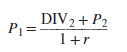
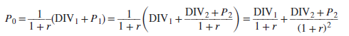
That is, a year from now, investors will be looking out at dividends in year 2 and price at the end of year 2. Thus, we can forecast P1 by forecasting DIV2 and P2, and we can express P0 in terms of DIV!, DIV2, and P2:
Take Fledgling Electronics. A plausible explanation for why investors expect its stock price to rise by the end of the first year is that they expect higher dividends and still more capital gains in the second. For example, suppose that they are looking today for dividends of $5.50 in year 2 and a subsequent price of $121. That implies a price at the end of year 1 of
![]()
Today’s price can then be computed either from our original formula
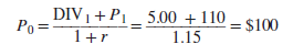
or from our expanded formula
![]()
We have succeeded in relating today’s price to the forecasted dividends for two years (DIV1 and DIV2) plus the forecasted price at the end of the second year (P2). You will not be surprised to learn that we could go on to replace P2 by (DIV3 + P3)/(1 + r) and relate today’s price to the forecasted dividends for three years (DIV1, DIV2, and DIV3) plus the forecasted price at the end of the third year (P3). In fact, we can look as far out into the future as we like, removing Ps as we go. Let us call this final period H. This gives us a general stock price formula:
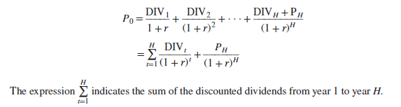
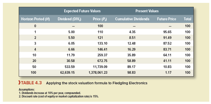
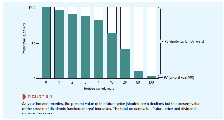
Table 4.3 continues the Fledgling Electronics example for various time horizons, assuming that the dividends are expected to increase at a steady 10% compound rate. The expected price Pt increases at the same rate each year. Each line in the table represents an application of our general formula for a different value of H. Figure 4.1 is a graph of the table. Each column shows the present value of the dividends up to the time horizon and the present value of the price at the horizon. As the horizon recedes, the dividend stream accounts for an increasing proportion of present value, but the total present value of dividends plus terminal price always equals $100.
How far out could we look? In principle, the horizon period H could be infinitely distant. Common stocks do not expire of old age. Barring such corporate hazards as bankruptcy or acquisition, they are immortal. As H approaches infinity, the present value of the terminal price ought to approach zero, as it does in the final column of Figure 4.1. We can, therefore, forget about the terminal price entirely and express today’s price as the present value of a perpetual stream of cash dividends. This is usually written as
![]()
where ro indicates infinity. This formula is the DCF or dividend discount model of stock prices. It’s another present value formula.[5] We discount the cash flows—in this case, the dividend stream—by the return that can be earned in the capital market on securities of equivalent risk. Some find the DCF formula implausible because it seems to ignore capital gains. But we know that the formula was derived from the assumption that price in any period is determined by expected dividends and capital gains over the next period.
Notice that it is not correct to say that the value of a share is equal to the sum of the discounted stream of earnings per share. Earnings are generally larger than dividends because part of those earnings is reinvested in new plant, equipment, and working capital. Discounting earnings would recognize the rewards of that investment (higherfuture earnings and dividends) but not the sacrifice (a lower dividend today). The correct formulation states that share value is equal to the discounted stream of dividends per share. Share price is connected to future earnings per share, but by a different formula, which we cover later in this chapter.
Although mature companies generally pay cash dividends, thousands of companies do not. For example, Amazon has never paid a dividend, yet it is a successful company with a market capitalization in January 2018 of $620 billion. Why would a successful company decide not to pay cash dividends? There are at least two reasons. First, a growing company may maximize value by investing all its earnings rather than paying out a dividend. The shareholders are better off with this policy, provided that the investments offer an expected rate of return higher than shareholders could get by investing on their own. In other words, shareholder value is maximized if the firm invests in projects that can earn more than the opportunity cost of capital. If such projects are plentiful, shareholders will be prepared to forgo immediate dividends. They will be happy to wait and receive deferred dividends.
The dividend discount model is still logically correct for growth companies, but difficult to use when cash dividends are far in the future. In this case, most analysts switch to valuation by comparables or to earnings-based formulas, which we cover in Section 4-4.
Second, a company may pay out cash not as dividends but by repurchasing shares from stockholders. We cover the choice between dividends and repurchases in Chapter 16, where we also explain why repurchases do not invalidate the dividend discount model.[7]
Nevertheless, the dividend discount model can be difficult to deploy if repurchases are irregular and unpredictable. In these cases, it can be better to start by calculating the present value of the total free cash flow available for dividends and repurchases. Discounting free cash flow gives the present value of the company as a whole. Dividing by the current number of shares outstanding gives present value per share. We cover this valuation method in Section 4-5.
The next section considers simplified versions of the dividend discount model.
I am incessantly thought about this, regards for posting.
Hello, i think that i saw you visited my web site so i came to “return the favor”.I’m attempting to find things to enhance my website!I suppose its ok to use a few of your ideas!!