Funds Outside the Security Market

Funds that are currently in the financial market are undoubtedly important, but the availability of funds outside the financial market also plays an important role in determining market conditions. The value of and the liquidity of household financial assets are important considerations when measuring how much money households might move into the securities markets. Money supply measures and bank loan activity are also important when considering how much money is available for the financial markets.

1. Household Financial Assets

Households, like corporations and governments, have different kinds of assets. They have both physical assets, such as cars and houses, as well as financial assets, such as stocks, bonds, mutual funds, and banking accounts. Some of their financial assets are liquid and some are not. Liquid assets can be converted to cash quickly; cash, bank deposits, money market mutual funds, U.S. Treasury bonds, notes, and bills are liquid financial assets. Other financial assets cannot always be converted to cash quickly; stocks generally are considered to be more liquid than other financial assets, such as pension funds, retirement accounts, profit­sharing accounts, unincorporated business ownership, trusts, mortgages, and life insurance.

A ratio of liquid financial assets to total financial assets shows how “liquid” households are—in other words, how easily they can raise cash if they need it. Generally, the more liquid households are, the more able they are to invest in stocks. When household liquidity is high, it is, therefore, favorable for the stock market, whereas low liquidity is negative for the stock market.

The data presented in Figure 10.3 from Ned Davis Research, Inc. shows a substantial decline in household liquidity in the 1990s and more recently since 2010. This is one reason why consumer debt has risen so strongly and why households are unable to withstand a severe economic contraction. During a severe economic contraction, one major source of funds for cash-strapped households is the stock market. Thus, this indicator, although it does not give mechanical signals, does measure the potential funds for stock demand or supply.

The range in percent of financial assets need not change by a large amount to have an effect on stock prices. According to a Ned Davis Research, Inc. study, when the percent of household financial assets has risen to 29.4%, the stock market has averaged an annual gain of 16.1%. A decline in percent to 25.4% corresponded with only a 3.2% gain in stock prices.

2. Money Supply (M 1 & M2)

Expansion in the money supply is a measure of potential demand for stock, as well as other assets, and is, thus, a rough measure of the potential for business and stock market expansion. Increases in the money supply have been historically associated with increases in economic growth and productivity. Although this economic theory is straightforward, quantifying actual money supply growth is not as easy as it seems. Measuring the amount of money in the economy depends on knowing what money is. If I ask you how much money you have, you would certainly count the currency and coins in your wallet. However, you would also probably think about the money you have in your checking account. Then, there is also the money you have in a savings account or money market mutual fund. Thus, the definition of money, and what to include in a measurement of money, is not as straightforward as it would initially seem.

The Federal Reserve measures money supply in a number of ways. Table 10.1 shows the various measurements of money that the Federal Reserve uses. The categories are based on liquidity, or the ease in which the financial assets can be converted into cash.

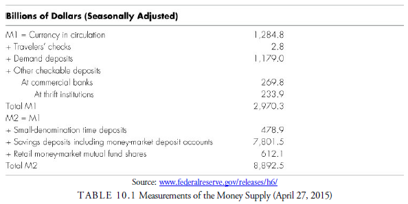
M1, the narrowest definition of money, is a measure of the most liquid assets in the financial system. It includes currency and the various deposit accounts on which individuals can write checks. M2 is a slightly broader measure of money, which includes M1 and various forms of savings accounts. The additional components of M2 are slightly less liquid than the financial assets of M1. Additional money sources not included in M1 or M2 are institutional money funds (1,781.6), foreign demand deposits in U.S. banks (88.9), foreign time and savings deposits (206.7), IRA and Keogh accounts (656.1), and U.S. government deposits (209.7) as of April 27, 2015. Today, the most commonly quoted monetary aggregate is M2 because its movements appear to be most closely related to interest rates and economic growth.

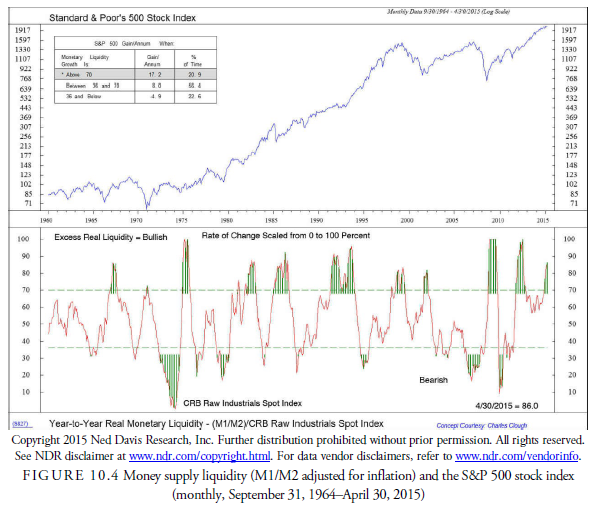
Because M1 is the most liquid portion of M2, a ratio of the two measures the liquidity of M2 and thus the proportion of M2 that can be used immediately for purchase of stocks and other investments. The Ned Davis Research, Inc. chart in Figure 10.4 shows the year-to-year change in this ratio scaled to between 0 and 100. Ned Davis Research, Inc. concluded that when the change advances above 70, the S&P 500 index gains at a rate of 17.2% per year, whereas when the change is 36 or below, the index declines at an annual rate of 4.9%. The liquidity of M2, therefore, is a powerful indicator of stock market direction.

3. Money Velocity

The velocity of money is a measure of how fast money turns over in the economy. It is calculated as a ratio of personal income to M2 (or sometimes GDP to M2). Money velocity is related to inflation; the faster money circulates, the more pressure that exists on prices, and the more it serves as a leading indicator of long­term interest rates, again because it reflects inflationary pressure. In terms of being an indicator for the stock market, Ned Davis Research, Inc. found that when money velocity (a monthly figure) rises above its 13- month moving average, the stock market has advanced 4.8% per annum on average. When money velocity declined below its 13-month moving average, the stock market advanced 9.1% per annum. This relationship is shown in Figure 10.5. Clearly, inflationary pressures from increased money velocity put a damper on stock market prices.

4. Yield Curve

The yield curve is a graphical representation of the yield on bonds with various lengths of time to maturity. The yield curve changes over time as short- and long-term interest rates change due to Federal Reserve action or the marketplace. Figure 10.6 shows the 3-month to 30-year yield curve at three different dates (May 31, 2014, November 30, 2014, and May 31, 2015) to display how the curve can change over a year’s time. Yield curve information is also summarized as a ratio or difference between a short-term and long­term interest rate over time. Figure 10.7 shows the difference between the long-term Treasury bond yield and the three-month Treasury bill rate from September 1964 through May 2015.

Banks traditionally practice maturity intermediation, borrowing short-term funds and lending to corporations or individuals over longer periods. Thus, they are said to “borrow short and lend long.” Their profit depends on the spread between the cost of funds, the short-term interest rate, and the return from loaned funds, the long-term interest rate. As short-term interest rates rise, presumably from Federal Reserve policy action, and long-term interest rates remain steady or decline, the yield curve becomes flatter and the banks are unable to profit as much from the spread. The yield curve, therefore, is a crude measurement of bank potential profitability. Bank profitability affects interest rates, and interest rates affect the stock market. Thus, the yield curve is a forecaster of stock market direction, and, historically, it has had an acceptable record of anticipating major turns in the stock market.

The “normal” relationship between interest-bearing instruments of the same quality is for longer rates to be higher than shorter rates. This is presumably because over time there is a risk of inflation, default, and other economic problems, the risk for which the holder of the long-term interest rate instrument wants to be compensated. This results in a positively sloped yield curve when plotting a graph with the time to maturity on the horizontal axis and the interest rate on the vertical axis for these securities.

The yield curve becomes abnormally steep when long-term rates rise considerably higher relative to short­term rates than the historic average of around 200 basis points. Although this can occur because of an upward movement in the long-term rate or a downward movement in the short-term rate, it is usually caused by the Fed lowering short-term rates to expand economic activity.

At times, short-term interest rates rise above long-term interest rates and the yield curve becomes inverted.

This inverted yield curve usually has dire consequences for the economy because it curtails the incentive of banks and other lending institutions that borrow money at short-term rates to make loans at long-term rates. The Federal Reserve estimates that an inverted yield curve predicts recessions two to six quarters ahead. Figure 10.7 shows the history of the yield curve and how it tends to forecast the direction of the stock market. Ned Davis Research found that when the long-rates advanced 1.1 percentage points above the short-rates, the stock market advanced 11.4% per annum on average. Contrarily, when the yield curve inverted, the stock market declined on average 7.2% per annum.

5. Bank Liquidity

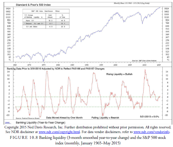
Generally, an increase in loan activity, the amount of loans being created and existing, is a sign of increased business activity. It can also be a sign of increased speculation or a particular period when banks, because the yield curve is so much in their favor, become less prudent in their lending policies. When loan demand increases, it puts upward pressure on interest rates. Conversely, a decrease in loan demand puts downward pressure on interest rates. One measure of bank speculation is the Liquidity Coverage Ratio (LCR). This ratio is the total of Category I financial assets, such as cash, gold bullion, and obligations of the U.S. government divided by the cash necessary to operate the bank for 30 days. Operation of the bank includes payroll, normal business expenses, payments on loans, and so on, that the bank incurs in its normal working mode. As the loan business gets hot, banks tend to loan right to the limit of their LCR. Thus, by following this estimate of bank liquidity, one can measure the risk of the banking system as well as the prospects for higher or lower interest rates. Ned Davis Research Inc., in Figure 10.8, displays a timing system based on the year-to-year change in bank liquidity that has shown excellent promise as a market timing device. It found that when the liquidity increases by 0.1 or more, the banks are becoming liquid and have the resources to lend. This is favorable for the economy and the stock market, which has gained 10.2% at an annual rate in such times. When the liquidity shrinks to -5.4 or below, the stock market declines at an annual rate of 4.8%. The liquidity year-to- year change is thus an excellent forecasting method for the stock market.

Source: Kirkpatrick II Charles D., Dahlquist Julie R. (2015), Technical Analysis: The Complete Resource for Financial Market Technicians, FT Press; 3rd edition.