Inferences About the Difference Between Two Population Means: Matched Samples

Suppose employees at a manufacturing company can use two different methods to per­form a production task. To maximize production output, the company wants to iden­tify the method with the smaller population mean completion time. Let m₁ denote the population mean completion time for production method 1 and m₂ denote the population mean completion time for production method 2. With no preliminary indication of the preferred production method, we begin by tentatively assuming that the two production methods have the same population mean completion time. Thus, the null hypothesis is H₀: μ₁ – μ₂ = 0. If this hypothesis is rejected, we can conclude that the population mean completion times differ. In this case, the method providing the smaller mean com­pletion time would be recommended. The null and alternative hypotheses are written as follows.

In choosing the sampling procedure that will be used to collect production time data and test the hypotheses, we consider two alternative designs. One is based on independent samples and the other is based on matched samples.

1. Independent sample design: A simple random sample of workers is selected and each worker in the sample uses method 1. A second independent simple random sample of workers is selected and each worker in this sample uses method 2. The test of the difference between population means is based on the procedures in Section 10.2.
2. Matched sample design: One simple random sample of workers is selected. Each worker first uses one method and then uses the other method. The order of the two methods is assigned randomly to the workers, with some workers performing method 1 first and others performing method 2 first. Each worker provides a pair of data values, one value for method 1 and another value for method 2.

In the matched sample design the two production methods are tested under similar con­ditions (i.e., with the same workers); hence this design often leads to a smaller sampling error than the independent sample design. The primary reason is that in a matched sample design, variation between workers is eliminated because the same workers are used for both production methods.

Let us demonstrate the analysis of a matched sample design by assuming it is the method used to test the difference between population means for the two production methods. A random sample of six workers is used. The data on completion times for the six workers are given in Table 10.3. Note that each worker provides a pair of data values, one for each production method. Also note that the last column contains the difference in completion times d_t for each worker in the sample.

The key to the analysis of the matched sample design is to realize that we consider only the column of differences. Therefore, we have six data values (.6, -.2, .5, .3, .0, and .6) that will be used to analyze the difference between population means of the two production methods.

Let μ_d = the mean of the difference in values for the population of workers. With this notation, the null and alternative hypotheses are rewritten as follows.

If H0 is rejected, we can conclude that the population mean completion times differ.

The d notation is a reminder that the matched sample provides difference data. The sample mean and sample standard deviation for the six difference values in Table 10.3 follow.

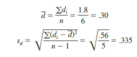
With the small sample of n = 6 workers, we need to make the assumption that the population of differences has a normal distribution. This assumption is necessary so that we may use the t distribution for hypothesis testing and interval estimation procedures. Based on this assump­tion, the following test statistic has a t distribution with n – 1 degrees of freedom.

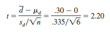
Let us use equation (10.9) to test the hypotheses H0: md = 0 and Ha: md Þ 0, using a = .05. Substituting the sample results d = .30, sd = .335, and n = 6 into equation (10.9), we compute the value of the test statistic.

Now let us compute the p-value for this two-tailed test. Because t = 2.20 > 0, the test statistic is in the upper tail of the t distribution. With t = 2.20, the area in the upper tail to the right of the test statistic can be found by using the t distribution table with degrees of freedom = n — 1 = 6 — 1 = 5. Information from the 5 degrees of freedom row of the t distribution table is as follows:

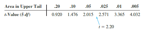
Thus, we see that the area in the upper tail is between .05 and .025. Because this test is a two-tailed test, we double these values to conclude that the p-value is between .10 and .05. This p-value is greater than a = .05. Thus, the null hypothesis H₀: Let us use equation (10.9) to test the hypotheses H0: md = 0 and Ha: md Þ 0, using a = .05.
Substituting the sample results d = .30, sd = .335, and n = 6 into equation (10.9), we
compute the value of the test statistic. μ_d = 0 is not rejected. Applying statistical software to the data in Table 10.3, we find the exact p-value = .080.

In addition, we can obtain an interval estimate of the difference between the two popula­tion means by using the single population methodology. At 95% confidence, the calculation follows.

Thus, the margin of error is .35 and the 95% confidence interval for the difference between the population means of the two production methods is — .05 minutes to .65 minutes.

Source:  Anderson David R., Sweeney Dennis J., Williams Thomas A. (2019), Statistics for Business & Economics, Cengage Learning; 14th edition.