Acceptance Sampling

In acceptance sampling, the items of interest can be incoming shipments of raw materi­als or purchased parts as well as finished goods from final assembly. Suppose we want to decide whether to accept or reject a group of items on the basis of specified quality characteristics. In quality control terminology, the group of items is a lot, and acceptance sampling is a statistical method that enables us to base the accept-reject decision on the inspection of a sample of items from the lot.

The general steps of acceptance sampling are shown in Figure 21.11. After a lot is received, a sample of items is selected for inspection. The results of the inspection are compared to specified quality characteristics. If the quality characteristics are satisfied, the lot is accepted and sent to production or shipped to customers. If the lot is rejected, man­agers must decide on its disposition. In some cases, the decision may be to keep the lot and remove the unacceptable or nonconforming items. In other cases, the lot may be returned to the supplier at the supplier’s expense; the extra work and cost placed on the supplier can motivate the supplier to provide high-quality lots. Finally, if the rejected lot consists of fin­ished goods, the goods must be scrapped or reworked to meet acceptable quality standards.

The statistical procedure of acceptance sampling uses the null and alternative hypotheses stated as follows:

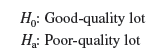
Table 21.4 shows the results of the hypothesis testing procedure. Note that correct decisions correspond to accepting a good-quality lot and rejecting a poor-quality lot.

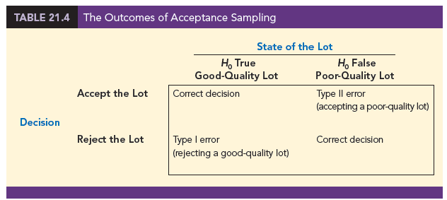
However, as with other hypothesis testing procedures, we need to be aware of the possibilities of making a Type I error (rejecting a good-quality lot) or a Type II error (accepting a poor-quality lot).

The probability of a Type I error creates a risk for the producer of the lot and is known as the producer’s risk. For example, a producer’s risk of .05 indicates a 5% chance that a good-quality lot will be erroneously rejected. The probability of a Type II error, on the other hand, creates a risk for the consumer of the lot and is known as the consumer’s risk. For example, a consumer’s risk of .10 means a 10% chance that a poor-quality lot will be erroneously accepted and thus used in production or shipped to the customer. Specific values for the producer’s risk and the consumer’s risk can be controlled by the person designing the acceptance sampling procedure. To illustrate how to assign risk values, let us consider the problem faced by KALI, Inc.

1. KALI, Inc.: An Example of Acceptance Sampling

KALI, Inc., manufactures home appliances that are marketed under a variety of trade names. However, KALI does not manufacture every component used in its products. Several components are purchased directly from suppliers. For example, one of the components that KALI purchases for use in home air conditioners is an overload protector, a device that turns off the compressor if it overheats. The compressor can be seriously damaged if the overload protector does not function properly, and therefore KALI is concerned about the quality of the overload protectors. One way to ensure quality would be to test every component received through an approach known as 100% inspection. However, to determine proper functioning of an overload protector, the device must be subjected to time-consuming and expensive tests, and KALI cannot justify testing every overload protector it receives.

Instead, KALI uses an acceptance sampling plan to monitor the quality of the overload protectors. The acceptance sampling plan requires that KALI’s quality control inspectors select and test a sample of overload protectors from each shipment. If very few defective units are found in the sample, the lot is probably of good quality and should be accepted. However, if a large number of defective units are found in the sample, the lot is probably of poor quality and should be rejected.

An acceptance sampling plan consists of a sample size n and an acceptance criterion c. The acceptance criterion is the maximum number of defective items that can be found in the sample and still indicate an acceptable lot. For example, for the KALI problem let us assume that a sample of 15 items will be selected from each incoming shipment or lot. Furthermore, assume that the manager of quality control states that the lot can be accepted only if no defective items are found. In this case, the acceptance sampling plan established by the quality control manager is n = 15 and c = 0.

This acceptance sampling plan is easy for the quality control inspector to implement. The inspector simply selects a sample of 15 items, performs the tests, and reaches a con­clusion based on the following decision rule.

• Accept the lot if zero defective items are found.
• Reject the lot if one or more defective items are found.

Before implementing this acceptance sampling plan, the quality control manager wants to evaluate the risks or errors possible under the plan. The plan will be implemented only if both the producer’s risk (Type I error) and the consumer’s risk (Type II error) are controlled at reasonable levels.

2. Computing the Probability of Accepting a Lot

The key to analyzing both the producer’s risk and the consumer’s risk is a “what-if ” type of analysis. That is, we will assume that a lot has some known percentage of defective items and compute the probability of accepting the lot for a given sampling plan. By vary­ing the assumed percentage of defective items, we can examine the effect of the sampling plan on both types of risks.

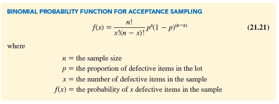
Let us begin by assuming that a large shipment of overload protectors has been received and that 5% of the overload protectors in the shipment are defective. For a shipment or lot with 5% of the items defective, what is the probability that the n = 15, c = 0 sampling plan will lead us to accept the lot? Because each overload protector tested will be either defective or nondefective and because the lot size is large, the number of defective items in a sample of 15 has a binomial distribution. The binomial probability function is as follows.

For the KALI acceptance sampling plan, n = 15; thus, for a lot with 5% defective (p = .05), we have

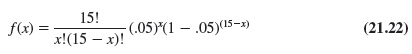
Using equation (21.22), f(0) will provide the probability that zero overload protectors will be defective and the lot will be accepted. In using equation (21.22), recall that 0! = 1.

Thus, the probability computation for ƒ(0) is

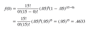
We now know that the n = 15, c = 0 sampling plan has a .4633 probability of accepting a lot with 5% defective items. Hence, there must be a corresponding 1 – .4633 = .5367 probability of rejecting a lot with 5% defective items.

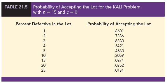
Excel’s BINOM.DIST function can be used to simplify making these binomial probabil­ity calculations. Using this function, we can determine that if the lot contains 10% defec­tive items, there is a .2059 probability that the n = 15, c = 0 sampling plan will indicate an acceptable lot. The probability that the n = 15, c = 0 sampling plan will lead to the acceptance of lots with 1%, 2%, 3%, . . . defective items is summarized in Table 21.5.

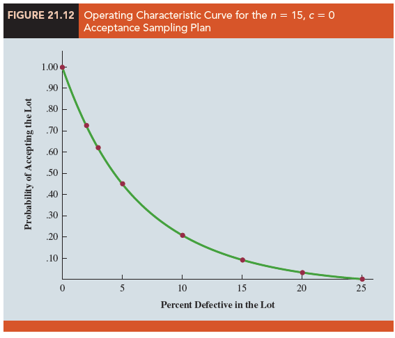
Using the probabilities in Table 21.5, a graph of the probability of accepting the lot versus the percent defective in the lot can be drawn as shown in Figure 21.12. This graph, or curve, is called the operating characteristic (OC) curve for the n = 15, c = 0 acceptance sampling plan.

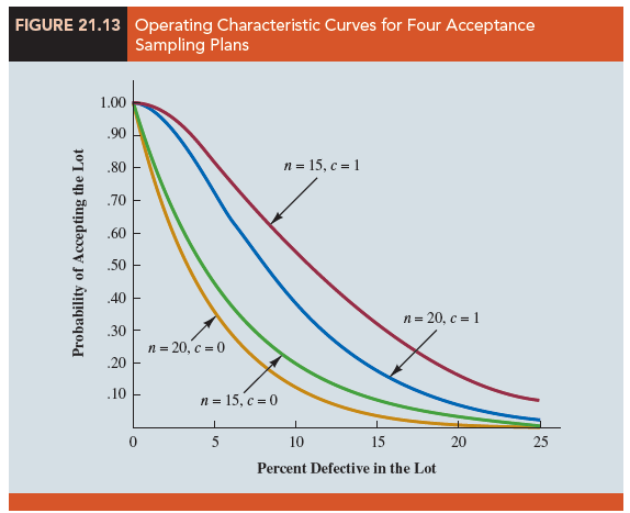
Perhaps we should consider other sampling plans, ones with different sample sizes n or different acceptance criteria c. First consider the case in which the sample size re­mains n = 15 but the acceptance criterion increases from c = 0 to c = 1. That is, we will now accept the lot if zero or one defective component is found in the sample. For a lot with 5% defective items (p = .05), the binomial probability function in equation (21.21) can be used to compute f(0) = .4633 and f(1) = .3658. Thus, there is a .4633 + .3658 = .8291 probability that the n = 15, c = 1 plan will lead to the acceptance of a lot with 5% defective items.

Continuing these calculations, we obtain Figure 21.13, which shows the operating characteristic curves for four alternative acceptance sampling plans for the KALI problem. Samples of size 15 and 20 are considered. Note that regardless of the proportion defective in the lot, the n = 15, c = 1 sampling plan provides the highest probabilities of accepting the lot. The n = 20, c = 0 sampling plan provides the lowest probabilities of accepting the lot; however, that plan also provides the highest probabilities of rejecting the lot.

3. Selecting an Acceptance Sampling Plan

Now that we know how to use the binomial distribution to compute the probability of accepting a lot with a given proportion defective, we are ready to select the values of n and c that determine the desired acceptance sampling plan for the application being studied.

To develop this plan, managers must specify two values for the fraction defective in the lot. One value, denoted p₀, will be used to control for the producer’s risk, and the other value, denoted p₁, will be used to control for the consumer’s risk.

We will use the following notation.

α = the producer’s risk; the probability of rejecting a lot with p₀ defective items

β = the consumer’s risk; the probability of accepting a lot with p₁ defective items

Suppose that for the KALI problem, the managers specify that p₀ = .03 and p₁ = .15. From the OC curve for n = 15, c = 0 in Figure 21.14, we see that p₀ = .03 provides a producer’s risk of approximately 1 – .63 = .37, and p₁ = .15 provides a consumer’s risk of approxi­mately .09. Thus, if the managers are willing to tolerate both a .37 probability of rejecting a lot with 3% defective items (producer’s risk) and a .09 probability of accepting a lot with 15% defective items (consumer’s risk), the n = 15, c = 0 acceptance sampling plan would be acceptable.

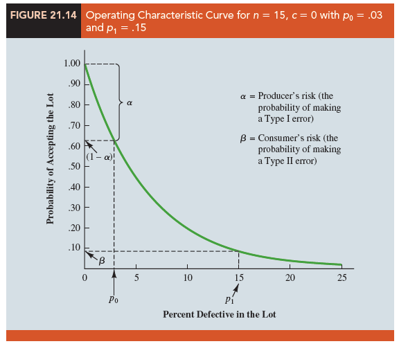
Suppose, however, that the managers request a producer’s risk of a = .10 and a consumer’s risk of b = .19. We see that now the n = 15, c = 0 sampling plan has a better-than-desired consumer’s risk but an unacceptably large producer’s risk. The fact that a = .37 indicates that 37% of the lots will be erroneously rejected when only 3% of the items in them are defective. The producer’s risk is too high, and a different acceptance sampling plan should be considered.

Using p₀ = .03, a = .10, p₁ = .15, and b = .20, Figure 21.13 shows that the acceptance sampling plan with n = 20 and c = 1 comes closest to meeting both the producer’s and the consumer’s risk requirements.

As shown in this section, several computations and several operating characteristic curves may need to be considered to determine the sampling plan with the desired produc­er’s and consumer’s risk. Fortunately, tables of sampling plans are published. For example, the American Military Standard Table, MIL-STD-105D, provides information helpful in designing acceptance sampling plans. More advanced texts on quality control, such as those listed in the bibliography, describe the use of such tables. The advanced texts also discuss the role of sampling costs in determining the optimal sampling plan.

4. Multiple Sampling Plans

The acceptance sampling procedure we presented for the KALI problem is a single-sample plan. It is called a single-sample plan because only one sample or sampling stage is used. After the number of defective components in the sample is determined, a decision must be made to accept or reject the lot. An alternative to the single-sample plan is a multiple sampling plan, in which two or more stages of sampling are used. At each stage a decision is made among three possibilities: stop sampling and accept the lot, stop sampling and reject the lot, or continue sampling. Although more complex, multiple sampling plans often result in a smaller total sample size than single-sample plans with the same a and b probabilities.

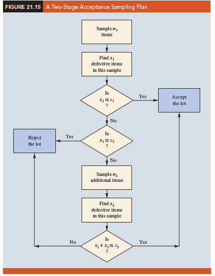
The logic of a two-stage, or double-sample, plan is shown in Figure 21.15. Initially a sample of n₁ items is selected. If the number of defective components x₁ is less than or equal to c₁, accept the lot. If x₁ is greater than or equal to c₂, reject the lot. If x₁ is between c₁ and c₂ (c₁ < x₁ < c₂), select a second sample of n₂ items. Determine the combined, or total, number of defective components from the first sample (x₁) and the second sample (x₂). If x₁ + x ₂ < c₃, accept the lot; otherwise reject the lot. The development of the double-sample plan is more difficult because the sample sizes n₁ and n₂ and the acceptance numbers c₁, c₂, and c₃ must meet both the producer’s and consumer’s risks desired.

Source:  Anderson David R., Sweeney Dennis J., Williams Thomas A. (2019), Statistics for Business & Economics, Cengage Learning; 14th edition.