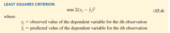
In Chapter 14, we used the least squares method to develop the estimated regression equation that best approximated the straight-line relationship between the dependent and independent variables. This same approach is used to develop the estimated multiple regression equation. The least squares criterion is restated as follows:
The predicted values of the dependent variable are computed by using the estimated multiple regression equation
![]()
As expression (15.4) shows, the least squares method uses sample data to provide the values of b0, b1, b2, • • • , bp that make the sum of squared residuals (the deviations between the observed values of the dependent variable (y;) and the predicted values of the dependent variable (y) a minimum.
In Chapter 14 we presented formulas for computing the least squares estimators b0 and b1 for the estimated simple linear regression equation y = b0 + b1x With relatively small data sets, we were able to use those formulas to compute b0 and b1 by manual calculations^ In multiple regression, however, the presentation of the formulas for the regression coefficients b0, b1, b2, • • • , bp involves the use of matrix algebra and is beyond the scope of this text Therefore, in presenting multiple regression, we focus on how statistical software can be used to obtain the estimated regression equation and other information The emphasis will be on how to interpret the computer output rather than on how to make the multiple regression computations^
1. An Example: Butler Trucking Company
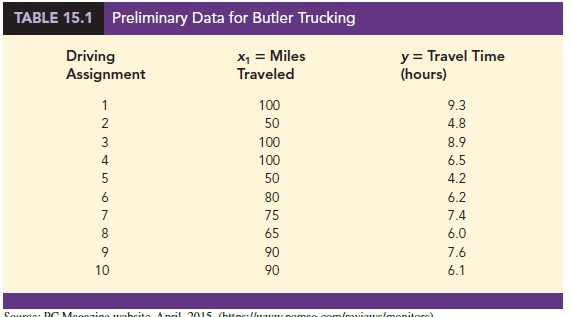
As an illustration of multiple regression analysis, we will consider a problem faced by the Butler Trucking Company, an independent trucking company in southern California^ A major portion of Butler’s business involves deliveries throughout its local area^ To develop better work schedules, the managers want to predict the total daily travel time for their driven
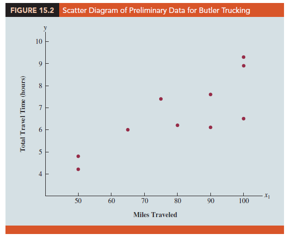
Initially the managers believed that the total daily travel time would be closely related to the number of miles traveled in making the daily deliveries^ A simple random sample of 10 driving assignments provided the data shown in Table 15T and the scatter diagram shown in Figure 15.2. After reviewing this scatter diagram, the managers hypothesized that the simple linear regression model y = β0 + β1x1 + e could be used to describe the relationship between the total travel time (y) and the number of miles traveled CyX To estimate the parameters β0 and β1, the least squares method was used to develop the estimated regression equatiom
![]()
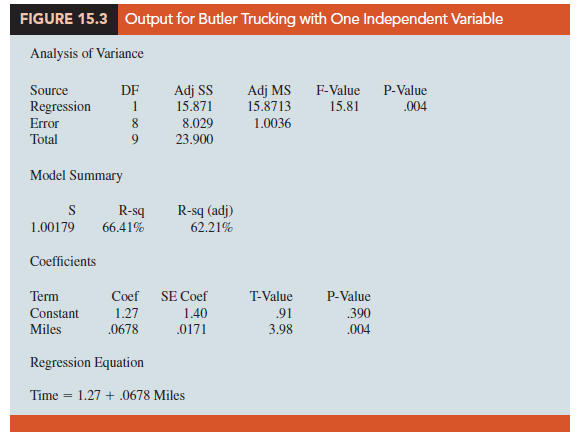
In Figure 153, we show statistical software output from applying simple linear regression to the data in Table 153^ The estimated regression equation is
![]()
At the 35 level of significance, the F value of 1531 and its corresponding p-value of 304 indicate that the relationship is significant; that is, we can reject H0: β1 = 0 because the p-value is less than a = .05. Note that the same conclusion is obtained from the t value of 3.98 and its associated p-value of .004. Thus, we can conclude that the relationship between the total travel time and the number of miles traveled is significant; longer travel times are associated with more miles traveled. With a coefficient of determination (expressed as a percentage) of R-Sq = 66.41%, we see that 66.41% of the variability in travel time can be explained by the linear effect of the number of miles traveled. This finding is fairly good, but the managers might want to consider adding a second independent variable to explain some of the remaining variability in the dependent variable.
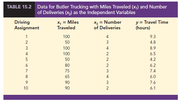
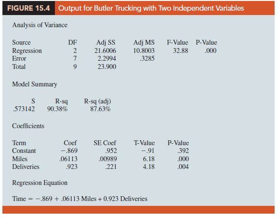
In attempting to identify another independent variable, the managers felt that the number of deliveries could also contribute to the total travel time. The Butler Trucking data, with the number of deliveries added, are shown in Table 15.2. Computer output with both miles traveled (x^ and number of deliveries (x2) as independent variables is shown in Figure 15.4. The estimated regression equation is
![]()
In the next section, we will discuss the use of the coefficient of multiple determination in measuring how good a fit is provided by this estimated regression equation. Before doing so, let us examine more carefully the values of b1 = .06113 and b2 = .923 in equation (15.6).
2. Note on Interpretation of Coefficients
One observation can be made at this point about the relationship between the estimated regression equation with only the miles traveled as an independent variable and the equation that includes the number of deliveries as a second independent variable. The value of b1 is not the same in both cases. In simple linear regression, we interpret b1 as an estimate of the change in y for a one-unit change in the independent variable. In multiple regression analysis, this interpretation must be modified somewhat. That is, in multiple regression analysis, we interpret each regression coefficient as follows: bt represents an estimate of the change in y corresponding to a one-unit change in xt when all other independent variables are held constant. In the Butler Trucking example involving two independent variables, b1 = .06113. Thus, .06113 hours is an estimate of the expected increase in travel time corresponding to an increase of one mile in the distance traveled when the number of deliveries is held constant. Similarly, because b2 = .923, an estimate of the expected increase in travel time corresponding to an increase of one delivery when the number of miles traveled is held constant is .923 hours.
Source: Anderson David R., Sweeney Dennis J., Williams Thomas A. (2019), Statistics for Business & Economics, Cengage Learning; 14th edition.
perfect review