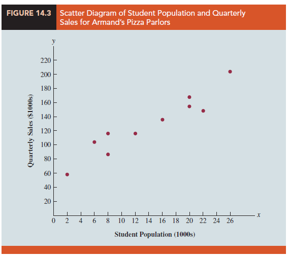
The least squares method is a procedure for using sample data to find the estimated regression equation. To illustrate the least squares method, suppose data were collected from a sample of 10 Armand’s Pizza Parlor restaurants located near college campuses. For the ith observation or restaurant in the sample, xi is the size of the student population (in thousands) and y is the quarterly sales (in thousands of dollars). The values of xi and y for the 10 restaurants in the sample are summarized in Table 14.1. We see that restaurant 1, with x1 = 2 and y1 = 58, is near a campus with 2000 students and has quarterly sales of $58,000. Restaurant 2, with x2 = 6 and y2 = 105, is near a campus with 6000 students and has quarterly sales of $105,000. The largest sales value is for restaurant 10, which is near a campus with 26,000 students and has quarterly sales of $202,000.
Figure 14.3 is a scatter diagram of the data in Table 14.1. Student population is shown on the horizontal axis and quarterly sales is shown on the vertical axis. Scatter diagrams for regression analysis are constructed with the independent variable x on the horizontal axis and the dependent variable y on the vertical axis. The scatter diagram enables us to observe the data graphically and to draw preliminary conclusions about the possible relationship between the variables.
What preliminary conclusions can be drawn from Figure 14.3? Quarterly sales appear to be higher at campuses with larger student populations. In addition, for these data the relationship between the size of the student population and quarterly sales appears to be approximated by a straight line; indeed, a positive linear relationship is indicated between x and y. We therefore choose the simple linear regression model to represent the relationship between quarterly sales and student population. Given that choice, our next task is to use the sample data in Table 14.1 to determine the values of b0 and b1 in the estimated simple linear regression equation. For the ith restaurant, the estimated regression equation provides

With yi denoting the observed (actual) sales for restaurant i and yt in equation (14.4) representing the predicted value of sales for restaurant i, every restaurant in the sample will have an observed value of sales yi and a predicted value of sales y. For the estimated regression line to provide a good fit to the data, we want the differences between the observed sales values and the predicted sales values to be small.
The least squares method uses the sample data to provide the values of b0 and b1 that minimize the sum of the squares of the deviations between the observed values of the dependent variable yi and the predicted values of the dependent variable y. The criterion for the least squares method is given by expression (14.5).

Differential calculus can be used to show (see Appendix 14.1) that the values of b0 and b1 that minimize expression (14.5) can be found by using equations (14.6) and (14.7).

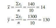
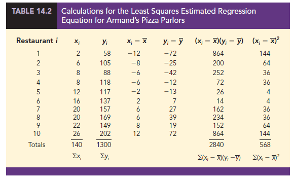
Some of the calculations necessary to develop the least squares estimated regression equation for Armand’s Pizza Parlors are shown in Table 14.2. With the sample of 10 restaurants, we have n = 10 observations. Because equations (14.6) and (14.7) require x and y we begin the calculations by computing x and y.
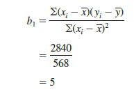
Using equations (14.6) and (14.7) and the information in Table 14.2, we can compute the slope and intercept of the estimated regression equation for Armand’s Pizza Parlors. The calculation of the slope (b1) proceeds as follows.
The calculation of the y intercept (b0) follows.
Thus, the estimated regression equation is
![]()
Figure 14.4 shows the graph of this equation on the scatter diagram.
The slope of the estimated regression equation (b1 = 5) is positive, implying that as student population increases, sales increase. In fact, we can conclude (based on sales measured in $1000s and student population in 1000s) that an increase in the student population of 1000 is associated with an increase of $5000 in expected sales; that is, quarterly sales are expected to increase by $5 per student.
If we believe the least squares estimated regression equation adequately describes the relationship between x and y, it would seem reasonable to use the estimated regression equation to predict the value of y for a given value of x. For example, if we wanted to predict quarterly sales for a restaurant to be located near a campus with 16,000 students, we would compute
![]()

Hence, we would predict quarterly sales of $140,000 for this restaurant. In the following sections we will discuss methods for assessing the appropriateness of using the estimated regression equation for estimation and prediction.
Source: Anderson David R., Sweeney Dennis J., Williams Thomas A. (2019), Statistics for Business & Economics, Cengage Learning; 14th edition.
Hi there! This post couldn’t be written any better! Reading through this post reminds me of my previous room mate! He always kept talking about this. I will forward this article to him. Pretty sure he will have a good read. Thank you for sharing!
I’m excited to find this page. I wanted to thank you for your time for this particularly wonderful read!! I definitely liked every little bit of it and I have you saved to fav to check out new things on your web site.