So far, we have discussed the demand curve for an individual consumer. Now we turn to the market demand curve. Recall from Chapter 2 that a market demand curve shows how much of a good consumers overall are willing to buy as its price changes. In this section, we show how market demand curves can be derived as the sum of the individual demand curves of all consumers in a particular market.
1. From Individual to Market Demand
To keep things simple, let’s assume that only three consumers (A, B, and C) are in the market for coffee. Table 4.2 tabulates several points on each consumer ’s demand curve. The market demand, column (5), is found by adding columns (2), (3), and (4), representing our three consumers, to determine the total quan- tity demanded at every price. When the price is $3, for example, the total quan- tity demanded is 2 + 6 + 10, or 18.
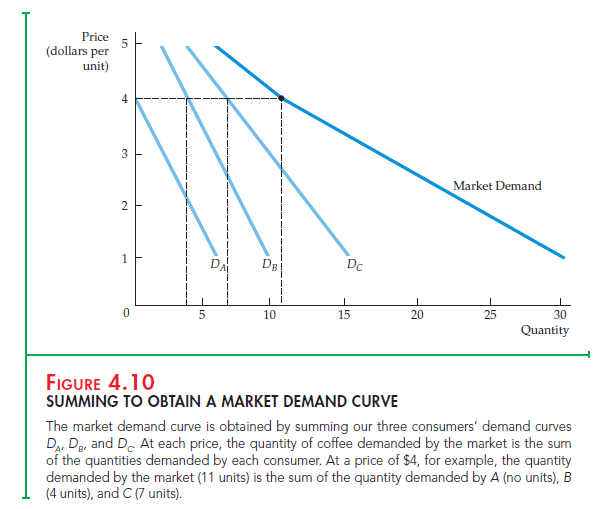
Figure 4.10 shows these same three consumers’ demand curves for coffee (labeled DA, DB, and DC). In the graph, the market demand curve is the horizon- tal summation of the demands of each consumer. We sum horizontally to find the total amount that the three consumers will demand at any given price. For
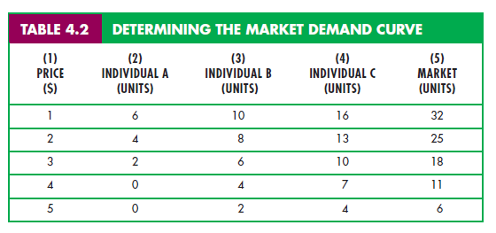
example, when the price is $4, the quantity demanded by the market (11 units) is the sum of the quantity demanded by A (no units), by B (4 units), and by C (7 units). Because all of the individual demand curves slope downward, the market demand curve will also slope downward. However, even though each of the individual demand curves is a straight line, the market demand curve need not be. In Figure 4.10, for example, the market demand curve is kinked because one consumer makes no purchases at prices that the other consumers find acceptable (those above $4).
Two points should be noted as a result of this analysis:
- The market demand curve will shift to the right as more consumers enter the market.
- Factors that influence the demands of many consumers will also affect market demand. Suppose, for example, that most consumers in a particular market earn more income and, as a result, increase their demands for cof- fee. Because each consumer ’s demand curve shifts to the right, so will the market demand curve.
The aggregation of individual demands into market demands is not just a theoretical exercise. It becomes important in practice when market demands are built up from the demands of different demographic groups or from consumers located in different areas. For example, we might obtain information about the demand for home computers by adding independently obtained information about the demands of the following groups:
- Households with children
- Households without children
- Single individuals
Or, we might determine U.S. wheat demand by aggregating domestic demand (i.e., by U.S. consumers) and export demand (i.e., by foreign consumers), as we will see in Example 4.3.
2. Elasticity of Demand
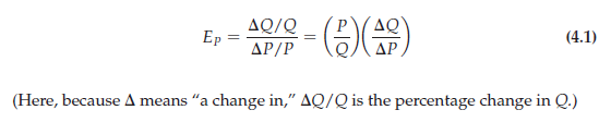
Recall from Section 2.4 (page 33) that the price elasticity of demand measures the percentage change in the quantity demanded resulting from a 1-percent increase in price. Denoting the quantity of a good by Q and its price by P, the price elasticity of demand is
INELASTIC DEMAND When demand is inelastic (i.e., Ep is less than 1 in absolute value), the quantity demanded is relatively unresponsive to changes in price. As a result, total expenditure on the product increases when the price increases. Suppose, for example, that a family currently uses 1000 gallons of gasoline a year when the price is $1 per gallon; suppose also that our family’s price elasticity of demand for gasoline is — 0.5. If the price of gasoline increases to $1.10 (a 10-percent increase), the consumption of gasoline falls to 950 gallons (a 5-percent decrease). Total expenditure on gasoline, however, will increase from $1000 (1000 gallons X $1 per gallon) to $1045 (950 gallons X $1.10 per gallon).
ELASTIC DEMAND In contrast, when demand is elastic (EP is greater than 1 in absolute value), total expenditure on the product decreases as the price goes up. Suppose that a family buys 100 pounds of chicken per year at a price of $2 per pound; the price elasticity of demand for chicken is —1.5. If the price of chicken increases to $2.20 (a 10-percent increase), our family’s consumption of chicken falls to 85 pounds a year (a 15-percent decrease). Total expenditure on chicken will also fall, from $200 (100 pounds * $2 per pound) to $187 (85 pounds * $2.20 per pound).

ISOELASTIC DEMAND When the price elasticity of demand is constant all along the demand curve, we say that the curve is isoelastic. Figure 4.11 shows an isoelastic demand curve. Note how this demand curve is bowed inward. In contrast, recall from Section 2.4 what happens to the price elasticity of demand as we move along a linear demand curve. Although the slope of the linear curve is constant, the price elasticity of demand is not. It is zero when the price is zero, and it increases in magnitude until it becomes infinite when the price is suffi- ciently high for the quantity demanded to become zero.
A special case of the isoelastic curve is the unit-elastic demand curve: a demand curve with price elasticity always equal to – 1, as is the case for the curve in Figure 4.11. In this case, total expenditure remains the same after a price change. A price increase, for instance, leads to a decrease in the quantity demanded that leaves the total expenditure on the good unchanged. Suppose, for example, that the total expenditure on first-run movies in Berkeley, California, is $5.4 million per year, regardless of the price of a movie ticket. For all points along the demand curve, the price times the quantity will be $5.4 million. If the price is $6, the quantity will be 900,000 tickets; if the price increases to $9, the quantity will drop to 600,000 tickets, as shown in Figure 4.11.
Table 4.3 summarizes the relationship between elasticity and expenditure. It is useful to review this table from the perspective of the seller of the good rather
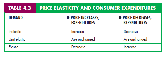
than the buyer. (What the seller perceives as total revenue, the consumer views as total expenditures.) When demand is inelastic, a price increase leads only to a small decrease in quantity demanded; thus, the seller ’s total revenue increases. But when demand is elastic, a price increase leads to a large decline in quantity demanded and total revenue falls.
Source: Pindyck Robert, Rubinfeld Daniel (2012), Microeconomics, Pearson, 8th edition.
I have found great messages right here. I enjoy the method you write.
So ideal!
I’m amazed, I have to admit. Rarely do I come across a blog that’s equally
educative and entertaining, and without a doubt, you’ve
hit the nail on the head. The problem is something that not enough
people are speaking intelligently about. I’m very happy I stumbled across this during my
hunt for something regarding this.
What’s up, yup this article is genuinely pleasant
and I have learned lot of things from it concerning
blogging. thanks.