Mediation, Moderation, and Canonical Correlation

1. Mediation

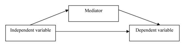
Mediation occurs when the observed relationship between two variables is due, at least in part, to a third variable. Statistically, mediation occurs when a variable (i.e., the mediating variable) reduces the magnitude of the relationship between two other variables. Mediation can be pictured as:

Conditions of Mediation

There are a few important conditions for statistical mediation. The mediating variable and the outcome variable should be continuous, a scale level variable (at least interval-level and normally distributed). This can be checked by using Frequencies and checking the skewness of the variable. The predictor variable in mediation in most studies is also a scale level variable, but it can also be dichotomous. If a dichotomous predictor variable is included, it is best to code it with “0” and “1” so that the regression equations are more easily interpreted. Multicollinearity can be a problem, so be sure to check for this.

In the past, some (e.g., Baron & Kenny, 1986) have stated that mediation can only occur if three conditions exist: (1) the predictor variable has a statistically significant correlation with the outcome variable, (2) the predictor variable has a statistically significant correlation with the mediating variable, and (3) the mediator variable has statistically significant correlations with both the predictor variable and the outcome variable. However, although this approach seems logical, mediation may exist even when the statistical association between some of these variables is not significant (Hayes, 2011), so requiring statistical significance may be unduly restrictive.

Assumptions of Mediation

The assumptions for mediation include the same assumptions as multiple regression including: that the relationship between each of the predictor variables and the dependent variable is linear and that the error, or residual, is normally distributed and uncorrelated with the predictors. Additionally, there are the assumptions that the variables have correct causal ordering and there is no reverse causality.

To test if the relationship between each of the predictor variables and the dependent variable is linear, scatterplots should be generated and checked. To test whether the error, or residual, is normally distributed and uncorrelated with the predictors, scatterplots of the errors should be checked. The assumptions of correct causal ordering and no reverse causality should be considered when designing the study and selecting variables for the analysis and, whenever possible, should be based on the empirical and theoretical literature. If using the PROCESS command, the assumptions need to be tested using Analyze ^ Regression ^ Linear. PROCESS is a macro that is added to SPSS manually using syntax commands. More about this can be found in how to run the Mediation analysis in SPSS using PROCESS when we compute a mediation analysis. Also, a matrix scatterplot needs to be created. See Chapter 6 for how to test the assumptions using these commands.

2. Moderation

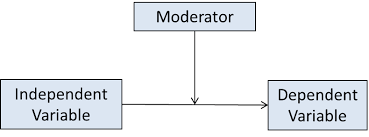
Moderation occurs when the relationship between two variables is different depending on the level of a third variable. For example, the relationship between motivation and math achievement may be greater for students who have high competence than for students who have low competence. Moderation can be pictured as:

Conditions of Statistical Moderation

There are a few conditions to consider when conducting moderation. The independent and outcome variable should be continuous; the moderating variable can be dichotomous or continuous. Dichotomous predictor variables need to have large samples within each group so that the sample means have narrow confidence intervals. Be sure to check for multicollinearity.

Assumptions of Statistical Moderation

The assumptions for moderation are the same as the assumption listed above for mediation.

See how to run the Moderation analysis in SPSS using PROCESS.

3. Canonical Correlation

In canonical correlation, you have two sets of two or more interval-level (scale) variables each and you want to see how differences in one set relate to differences in the other set of variables. With canonical correlation, unlike regression, there is no distinction between independent and dependent variables; they are called by SPSS “Set 1” and “Set 2.” One would use canonical correlation when the variables in each set can be grouped together conceptually, but you want to see if there are particular subsets of them that relate to subsets in the other variable set, so you do not want to sum each set to make an overall score. For example, one might wish to relate a set of child behavior variables to a set of parent behavior variables. One might wish to see which subset of parenting variables is associated with which subsets of child behavior variables. Usually, canonical correlation is used as an exploratory technique; it is not commonly used to test specific hypotheses. Like principal components analysis, canonical correlation enables you to see which variables go together; however, it does so in terms of how well the variables from Set 1 relate to those from Set 2. It determines which subset of the “Set 1” variables maximally relate to the “Set 2” variables, then which other subset of the “Set 1” variables relate to another subset of the “Set 2” variables, etc. (Note: For those of you using earlier versions of SPSS, it has been reported that SPSS versions below 10.0 tend to have problems running canonical correlations. If you are using an earlier version and have problems, check the Help menu.)

Conditions of Canonical Correlation

All variables in canonical correlation must be scale. It is recommended to have at least 10 subjects per variable in order to have adequate power.

Assumptions of Canonical Correlation

The assumptions of canonical correlation include: linearity of relationship (between each variable pair as well as between the variables and the linear composites), multivariate normality, and homoscedasticity. Because multivariate normality is difficult to assess, univariate normality can be evaluated. Multicollinearity should be assessed as well. All of the assumptions can be evaluated through a matrix scatterplots that can be generated using the MANOVA command.

Source: Leech Nancy L. (2014), IBM SPSS for Intermediate Statistics, Routledge; 5th edition;

download Datasets and Materials.