Simple Linear Regression Model

Armand’s Pizza Parlors is a chain of Italian-food restaurants located in a five-state area. Armand’s most successful locations are near college campuses. The managers believe that quarterly sales for these restaurants (denoted by y) are related positively to the size of the student population (denoted by x); that is, restaurants near campuses with a large student population tend to generate more sales than those located near campuses with a small stu­dent population. Using regression analysis, we can develop an equation showing how the dependent variable y is related to the independent variable x.

1. Regression Model and Regression Equation

In the Armand’s Pizza Parlors example, the population consists of all the Armand’s restau­rants. For every restaurant in the population, there is a value of x (student population) and a corresponding value of y (quarterly sales). The equation that describes how y is related to x and an error term is called the regression model. The regression model used in simple linear regression follows.

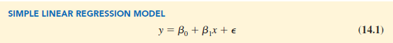
β₀ and β₁ are referred to as the parameters of the model, and e (the Greek letter epsilon) is a random variable referred to as the error term. The error term accounts for the variability in y that cannot be explained by the linear relationship between x and y.

The population of all Armand’s restaurants can also be viewed as a collection of subpop­ulations, one for each distinct value of x. For example, one subpopulation consists of all Ar­mand’s restaurants located near college campuses with 8000 students; another subpopulation consists of all Armand’s restaurants located near college campuses with 9000 students; and so on. Each subpopulation has a corresponding distribution of y values. Thus, a distribution of y values is associated with restaurants located near campuses with 8000 students; a distribu­tion of y values is associated with restaurants located near campuses with 9000 students; and so on. Each distribution of y values has its own mean or expected value. The equation that describes how the expected value of y, denoted E(y), is related to x is called the regression equation. The regression equation for simple linear regression follows.

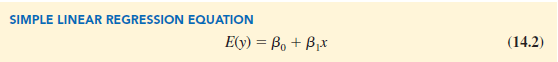
The graph of the simple linear regression equation is a straight line; β₀ is the y-intercept of the regression line, β₁ is the slope, and E(y) is the mean or expected value of y for a given value of x.

Examples of possible regression lines are shown in Figure 14.1. The regression line in Panel A shows that the mean value of y is related positively to x, with larger values of E(y) associated with larger values of x. The regression line in Panel B shows the mean value of y is related negatively to x, with smaller values of E(y) associated with larger values of x. The regression line in Panel C shows the case in which the mean value of y is not related to x; that is, the mean value of y is the same for every value of x.

2. Estimated Regression Equation

If the values of the population parameters β₀ and β₁ were known, we could use equation (14.2) to compute the mean value of y for a given value of x. In practice, the parameter values are not known and must be estimated using sample data. Sample statistics (denoted β₀ and β₁) are computed as estimates of the population parameters β₀ and β₁. Substituting the values of the sample statistics b₀ and β₁ for β₀ and β₁ in the regression equation, we obtain the estimated regression equation. The estimated regression equation for simple linear regression follows.

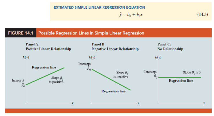
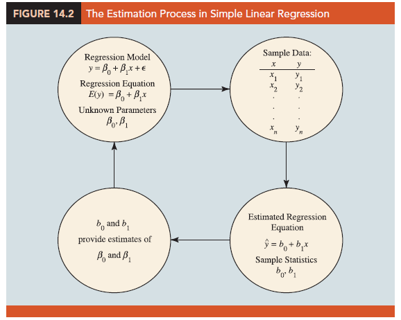
Figure 14.2 provides a summary of the estimation process for simple linear regression.

The graph of the estimated simple linear regression equation is called the estimated regression line; b₀ is the y-intercept and b₁ is the slope. In the next section, we show how the least squares method can be used to compute the values of b₀ and b₁ in the estimated regression equation.

In general, y is the point estimator of E(y), the mean value of y for a given value of x. Thus, to estimate the mean or expected value of quarterly sales for all restaurants located near campuses with 10,000 students, Armand’s would substitute the value of 10,000 for x in equation (14.3). In some cases, however, Armand’s may be more inter­ested in predicting sales for one particular restaurant. For example, suppose Armand’s would like to predict quarterly sales for the restaurant they are considering building near Talbot College, a school with 10,000 students. As it turns out, the best predictor of y for a given value of x is also provided by y. Thus, to predict quarterly sales for the restaurant located near Talbot College, Armand’s would also substitute the value of 10,000 for x in equation (14.3).

Source:  Anderson David R., Sweeney Dennis J., Williams Thomas A. (2019), Statistics for Business & Economics, Cengage Learning; 14th edition.