Principal Component Analysis and Principal Component Factoring by using Stata

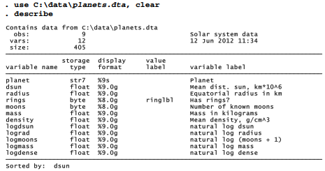
To illustrate principal component and factor analysis, we start with the small dataset, planets.dta, describing the nine classical planets of this solar system (from Beatty et al. 1981). The data include several variables in both raw and natural logarithm form. Logarithms are employed here to reduce skew and linearize relationships among the variables.

Principal component analysis finds the linear combination that explains the maximum amount of variance among the observed variables — called the “first principal component.” It also finds another, orthogonal (uncorrelated) linear combination that explains the maximum amount of remaining variance (“second principal component”), and so on until all variance is explained. From k variables we extract k principal components, which between them explain all of the variance. Principle component analysis serves as a data reduction technique because fewer than k components will often explain most of the observed variance. If further work concentrates on those components, the analysis can be simplified.

Applied to six variables describing the planets, we get six principal components that explain all the variance:

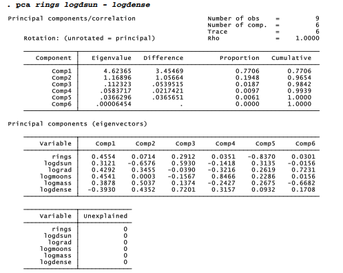
The pca output tells us that together, the first two components explain more than 96% of the cumulative variance of all six variables. Eigenvalues correspond to the standardized variance explained by each component. With six variables, the total standardized variance is 6. Of this, we see that component 1 explains 4.62365, which amounts to 4.62365/6 = .7706 or about 77% of the total. Component 2 explains 1.16896/6 = .1948, or an additional 19%. Principal components having eigenvalues below 1.0 are explaining less than the equivalent of one variable’s variance, which makes them unhelpful for data reduction. Analysts commonly set aside minor components and focus on those that have eigenvalues of at least one.

A good way to proceed with such data reduction is through the factor command, which offers principal component factoring as one of its options. To obtain principal component factors, type

Principal component factoring starts with extraction of principal components, but then retains only those that meet criteria for importance — by default, those with eigenvalues above 1. As we saw in the earlier pca example, only the first two components here meet that criterion, and together explain over 96% of the six variables’ combined variance. The unimportant 3rd through 6th principal components can safely be disregarded.

Two factor options provide control over the number of factors extracted:

factors(#)          where # specifies the number of factors

mineigen(#)       where # specifies the minimum eigenvalue for retained factors

Because principal component factoring automatically drops factors with eigenvalues below 1,

. factor rings logdsun – logdense, pcf

is equivalent to

. factor rings logdsun – logdense, pcf mineigen(l)

In this example, we would also have obtained the same results by typing

. factor rings logdsun – logdense, pcf factors(2)

To see a scree graph (plot of eigenvalues versus component or factor number) after any factor, use the screeplot command. A horizontal line at eigenvalue = 1 in Figure 11.1 marks the usual cutoff for retaining principal components, and again emphasizes the unimportance of components 3 through 6.

Source: Hamilton Lawrence C. (2012), Statistics with STATA: Version 12, Cengage Learning; 8th edition.