Simultaneous Equations Models by using EViews

1. EXAMINING THE DATA

In this section, the text introduces a two-equation demand and supply model for truffles, a French gourmet mushroom delicacy. To estimate the truffles model in EViews, open the workfile truffles.wfl. Open a Group containing the data. While holding down the Ctrl-key, select P, Q, PS, DI and PF. The first few observations look like

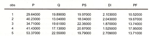
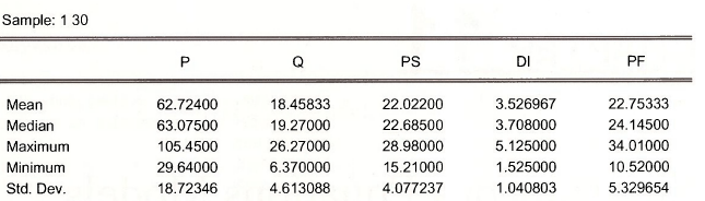
The summary statistics for the variables are obtained from the spreadsheet by selecting View/Descriptive Stats/Common Sample

2. ESTIMATING THE REDUCED FORM

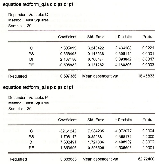
We first estimate the reduced form equations of POE Section 11.6.2 by regressing each endogenous variable, Q, and P, on the exogenous variables, PS, DI, and PF. We can quickly accomplish this task with the following statements typed in the EViews command window. The results match those in POE Table 11.2, page 313.

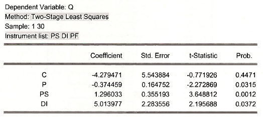
3. TSLS ESTIMATION OF AN EQUATION

Any identified equation within a system of simultaneous equations can be estimated by two-stage least squares (2SLS/TSLS). Click on Quick/Estimate Equation.

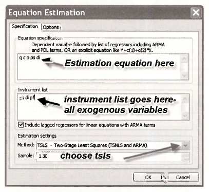
To estimate the demand equation by 2SLS select the method to be TSLS, and fill in the demand equation variables in Equation specification, the upper area of the dialog box, and list all the exogenous variables in the system in the Instrument list. Click OK. Name the resulting equation DEMAND.

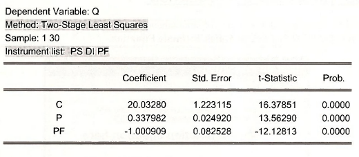
To estimate the supply equation we illustrate the use of the command line,

equation supply.tsls q c p pf @ ps di pf

In this command we name the estimation SUPPLY and the estimation technique TSLS by equation supply.tsls. The specification of the equation if followed by the instrumental variables, which follow @.

 4. TSLS ESTIMATION OF A SYSTEM OF EQUATIONS

As noted in Section 11.2 we can apply TSLS equation by equation for all the identified equations within a system of equations. If all the equations in the system are identified, then all the equations can be estimated in one step.

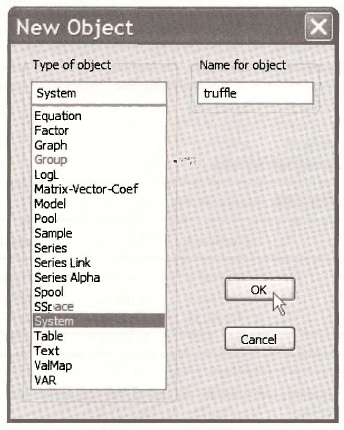
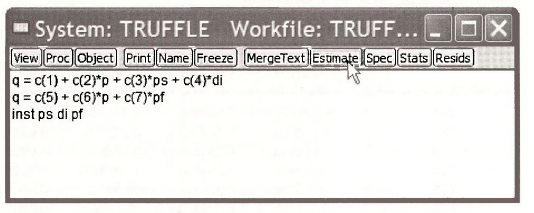
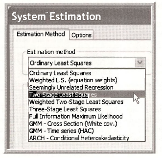
We introduce a new EViews object here: the SYSTEM. From the EViews menubar, click on Objects/New Object, select System, name the system object TRUFFLE, and click OK.

Next, enter the system equation specification given in POE equations (11.1) and (11.2), on page 304. Note that you must enter a line that contains the exogenous (determined outside the model) variables in the system, PS, Dl, and PF. In the context of two-stage least squares estimation of our truffles system, EViews refers to these exogenous variables as “instruments”. Enter the line INST PS DI PF directly below the supply equation, and click Estimate on the system’s toolbar.

To reproduce the results found in Tables 11.3a and 11.3b in your text, under Estimation Method, check the Two-Stage Least Squares checkbox, and click OK.

The results, on the following page, are identical to the equation by equation approach of estimating demand and then supply, but this system estimation approach opens the window to many advanced procedures that you may learn about in subsequent econometrics courses.

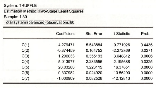
At the bottom of the System Table we find each equation represented and summarized.

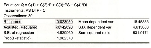
Note in these results that R² and adjusted-R² are negative. This is not uncommon when using generalized least squares, instrumental variables or two-stage least squares. For any estimator but least squares, the identity SST = SSR + SSE does not hold, so the usual R² = 1 – SSE/SST can produce negative numbers. This just shows that the goodness-of-fit measure is not appropriate in this context, and should be ignored.

5. SUPPLY AND DEMAND AT FULTON FISH MARKET

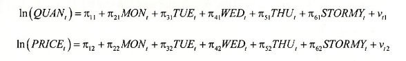
A second example of a simultaneous equations model is given by the Fulton Fish Market discussed in POE Section 11.7, page 314. Open the workfile fultonfish.wfl. Let us specify the demand equation for this market as

Where QJJAN_t is the quantity sold, in pounds, and PRICE_t the average daily price per pound. Note that we are using the subscript “r to index observations for this relationship because of the time series nature of the data. The remaining variables are dummy variables for the days of the week, with Friday being omitted. The coefficient a₇ is the price elasticity of demand, which we expect to be negative. The daily dummy variables capture day to day shifts in demand. The supply equation is

The coefficient β₂ is the price elasticity of supply. The variable STORMY is a dummy variable indicating stormy weather during the previous three days. This variable is important in the supply equation because stormy weather makes fishing more difficult, reducing the supply of fish brought to market.

The reduced form equations specify each endogenous variable as a function of all exogenous variables

The least squares estimates of the reduced forms are given by

Is Iquan c mon tue wed thu stormy

Is Iprice c mon tue wed thu stormy

The key reduced form equation is the second, for 1 n(PRICE).

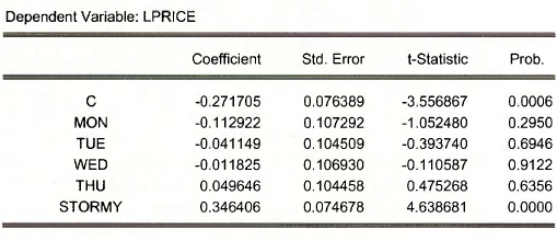
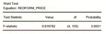
See POE pages 316-317 for a discussion of the importance of the strong significance of the variable STORMY and the lack of the significance of the day dummies, individually or jointly.

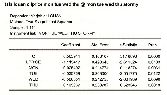
The TSLS estimates of the demand equation in POE Table 11.5, page 317, are obtained using

Source: Griffiths William E., Hill R. Carter, Lim Mark Andrew (2008), Using EViews for Principles of Econometrics, John Wiley & Sons; 3rd Edition.