Dynamic Models, Autocorrelation, and Forecasting by using EViews

1. LEAST-SQUARES RESIDUALS: SUGARCANE EXAMPLE

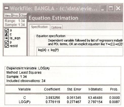
The first example considered in Chapter 9 is an area response model for sugarcane in Bangladesh where area sown to sugarcane A is related to price P by the equation

In contrast to earlier chapters where the index used for the observations was mainly i, here we use the index t to denote time-series observations. We have 34 annual observations stored in the fde bangla.wfl. The Equation specification and resulting least-squares output are

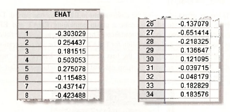
We are interested in examining the residuals from this estimated equation, as displayed in Table 9.1 on page 233 of the text. Various ways of examining the residuals were described at the beginning of Chapter 8. As a first step for this example, we save them and then check them against the values that appear in Table 9.1. The command series ehat = resid saves the residuals as To view them double click on EHAT and select View/SpreadSheet. The first and last 8 values are as follows.

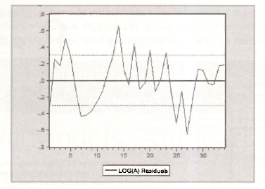
A plot of the residuals against time can indicate whether positive residuals tend to follow positive residuals and negative residuals tend to follow negative residuals – a sign of positive autocorrelation. To obtain the plot in Figure 9.3 open the least-squares estimated equation and go to View/Actual, Fitted, Residual/Residual Graph. The following graph appears.

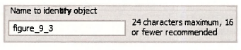
To save this graph in your workfile, click on [Freeze 1 and then [Name! and enter a suitable name.

There are other ways to create this graph. For example, you could open the series EHAT and then select View/Graph/Basic graph/Line & Symbol. Clicking OK will produce the graph. If you then follow up by clicking [Freeze], you will be able to edit and save the graph.

1.1. Correlation between e_t and e_t-1

The sample correlation between the least squares residuals e_t and their lagged values e,_,, is an important quantity for assessing whether or not the equation errors are autocorrelated. To compute this quantity we begin by creating the variable e. , and giving it the name EHAT_1. The EViews command is

series ehat_1 =ehat(-1)

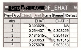
Writing ehat(-1) has the effect of lagging the observations in EHAT by one period. To appreciate how lagged observations are stored, we create a group containing EHAT and EHAT_1 and examine the first few observations in the spreadsheet. They are illustrated on the following page. Notice what has happened. The 2nd observation for EHAT_1 is e,, the 3rd observation is e₂, and so on. Because there is no observation e₀, the first observation on EHAT_1 is “not available” and is recorded as NA. When asked to perform calculations that include this first observation, EViews will omit it.

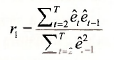
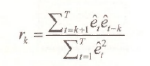
Now consider the first-order correlation r, given in equation (9.18) on page 234 of the text

The numerator and denominator of this quantity can be computed using the following commands

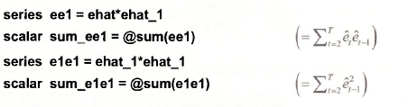
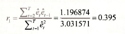
We have created two new series, e_te_t-1 and e²_t-1, and then found their sum. The first observation in each of the series EE1 and E1E1 will be NA. The values obtained for their sums are , leading to a value for r₁ of

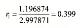
This value differs slightly from that reported in the text which is r₁ – 0.404. The text value was obtained using the EViews command

scalar r1_text = @cor(ehat, ehat_1)

where @cor(x1,x2) is the EViews function for computing the correlation between two series XI and X2. The reason for the discrepancy is that, after omitting the first observation (or the last observation), the sample mean for e_t is no longer zero. The formula used by the @cor function is

where e_[-1] is the sample mean of the e_t, with the first observation excluded and e_[-_T] is the sample mean of the e_t, with the last observation excluded. In general the difference between the two alternative formulas will be slight and it disappears as the sample size gets larger.

If having two different formulas for r₁ worries you, it may help to remember that they are simply two alternative estimators for the population correlation between the error and its lag

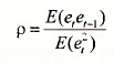
Having different estimators for the same population quantity is not unusual. The least squares and generalized least squares estimators in Chapter 8 are examples.

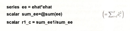
Now that you are comfortable with the idea of two estimators for the same population quantity, it is convenient to introduce one more. A 3rd estimator for p is relevant later in this chapter when we explain how EViews computes a sample correlogram. When sample size is large, the difference between it and the other estimators will be negligible. Its formula and value for the sugarcane residuals are

Notice that the denominator includes all observations on e . We can use EViews to compute this version of q as follows.

2. NEWEY-WEST STANDARD ERRORS

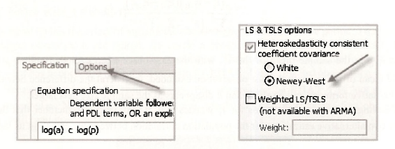
In Chapter 8 when studying heteroskedasticity, we saw how least squares could be used instead of generalized least squares as long as we used White standard errors. A similar option exists for regression models with autocorrelated errors. In this case the standard errors are called Newey- West or HAC standard errors, with HAC being an acronym for heteroskedasticity-autocorrelation consistent. To compute the Newey-West standard errors for the sugarcane example, as reported on page 235 of the text, we choose Options in the Equation Estimation window. Then, in the Options window, go to the LS & TSLS options section, tick the Heteroskedasticity consistent coefficient covariance box, and select Newey-West. The Newey-West standard errors are consistent under both heteroskedasticity and autocorrelation.

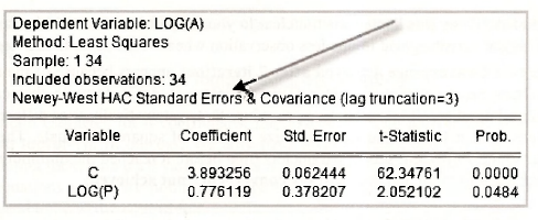
The least-squares output with the corrected standard errors follows. Notice that Eviews has a note to tell you that it has calculated Newey-West standard errors.

3. ESTIMATING AN AR(1) ERROR MODEL

Continuing with the sugar cane example, we are interested in estimating the supply equation under the assumption that the errors follow an AR(1) model. These two components of the model can be written as

3.1. A short way

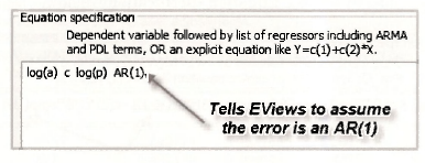
To estimate a model with an AR(1) error we begin, as usual, by selecting Object/New Object/ Equation. After giving the equation object a name and clicking OK, the Equation specification box appears. Then, as before, you enter the names of the series that are in the equation, but this time you also add AR(1) to tell EViews the errors follow an AR(1) model.

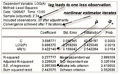
You will notice several new features in the output that follows.

An estimate p = 0.42214 is provided next to the name AR(1).
The E of regression is the estimate a_v = 0.2854 .
The lagged variables in the equation lead to a loss of one observation. EViews automatically changes the Sample from 1 34 to 2 34, and reports that 33 observations are included. If why this happens is not clear to you, be patient. More will be said about how the lagged variables lead to one less observation when we move on to the “long way”.

The note Convergence achieved after 7 iterations appears because of the nature of the nonlinear least squares estimator. This estimator is not a formula that calculates the required numbers. It is an iterative procedure that systematically tries different parameter values until it finds those that minimize the sum of squared residuals. The 7 iterations refer to the 7 different sets of parameters tried before it reached the minimum. If it fails to reach the minimum, the note will say convergence not achieved.

3.2. A long way

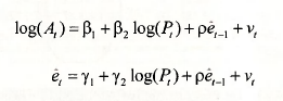
An alternative way of writing the AR(1) error model is

See page 236 of the text for a derivation of this result. We have made the substitutions y_t =ln(A_t) and x_t =ln(P_t). Using C(1) = β₁, C(2) = β₂ and C(3) = p, this equation can be estimated by writing it directly into the Equation specification window.

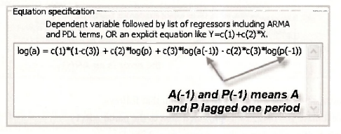
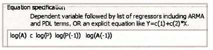
Can you see what is different? Instead of writing in the name of the dependent variable followed by the explanatory variables, we have written out the whole equation. Also, the EViews notation for A_t-1, and P , is a(-1) and p(-1), respectively. What would happen if we tried to estimate the equation using

log(a) c log(p) log(a(-1)) log(p(-1))

We would obtain estimates for 4 coefficients, one associated with each of the series c, log(p), log(a(-1)), and >og(p(-l)). In our case we only have 3 coefficients, and there is not an obvious way of associating them with each variable. This is the reason for writing out the equation in full. In general, equations which are nonlinear in the coefficients or that involve restrictions on the coefficients need to be written out in full.

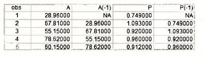
It is useful to examine the lagged variables A_t-1 = a(-1) and P_t-1 = p(-1) in more detail. The following spreadsheet contains the first 5 observations on A_t, A_t-1, P_t and P_t-1 Notice that lagging has the effect of making the first observations for A_t-1, and P_t-1 not available. Accordingly, EViews omits it when carrying out estimation.

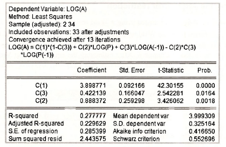
The output appears below. The first thing you should notice in this output is that the results are identical to those obtained the “short way”. The equation specifications for the short way and the long way are two different ways of telling EViews to do the same thing, namely, find values for β₁, β₂ and p that minimize

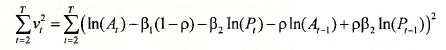
Notice also that the sample has been adjusted to omit the first observation, convergence took 13 iterations in this case, and EViews writes out the equation that has been estimated so that you can readily see where each of the coefficients appears in the equation.

3.3. A more general model

In the previous section we asked what would happen if we used the following Equation specification

In this case we are estimating the model

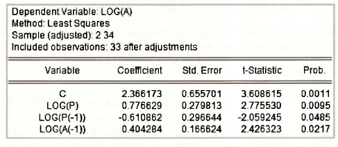
This model has the same variables as the AR(1) error model of the previous section, but it has 4 coefficients instead of 3. It is a more general model, known as an ARDL(1,1) model, that reduces to the AR(1) error model when δ₁ = -θ₁δ₀. ARDL models are discussed later in this chapter. The results below appear in equation (9.28) on page 239 of the text.

3.4. Testing the AR(1) error restriction

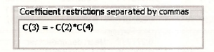
The restriction δ₁ = -θ₁δ₀ can be tested using a Wald test with hypotheses H₀:δ₁ = -θ₁δ₀ and H₁ : δ₁ # -θ₁δ₀. It differs from the Wald tests we considered in Chapter 6 because the hypothesis is a nonlinear function of the coefficients. Nevertheless, EViews can perform the test using the same procedures described in Chapter 6. After estimating the equation, select View/Coefficient TestsAVald Coefficient Restrictions. Recognizing that C(2) = δ₀, C(3) = δ₁, and C(4)= θ₁, the null hypothesis is entered in the Wald Test dialog box as follows

Clicking OK, yields the following test output.

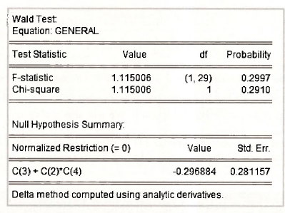
The test is performed in the same way as described in Chapter 6, although, because of the nonlinearity of the hypothesis, the formulas for the F- and x²- statistics are different. These formulas as well as the delta method that is used to compute se(δ₁ + θ₁δ₀) = 0.281157 are things that you will leam in a later stage of your econometric career. Since p-value = 0.29 > 0.05 , we do not reject the restriction implied by the AR(1) error model. In this case the normalized restriction is 8, + O^ = 0 and its estimated left hand side is δ₁ + θ₁δ₀ = -0.296884.

4. TESTING FOR AUTOCORRELATION

4.1. Residual correlogram

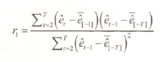
Autocorrelation exists when the equation error e_t is correlated with any of its past values e_t–₁,e_t–₂,…. One way to investigate the possible existence of such correlation is to obtain the least squares residuals e_t and to check whether the sample correlations between e_t, and e_t_₁, e_t_₂are significantly different from zero. The sequence of these correlations r₁,r₂,… is called the residual correlogram. Earlier in this chapter (Section 9.1.1) we saw that there are three slightly different formulas for computing r₁. Consider the correlation at a general lag k. The formula that EViews uses for computing r_k (the correlation between e_t and e_t-k) is

Another possible formula omits the last k terms in the summation in the denominator which then becomes . A third alternative is the EViews function @cor(e, ,e,.,). It computes a mean-corrected version whose formula is

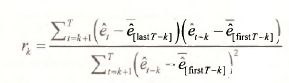
where e_[last_T__k] is the sample mean of the e_t for the last T-k observations, and e_[first_T._k] is the sample mean of the e_t for the first T-k observations. In what follows we will report the EViews residual correlogram and describe how to obtain it. We will also explain any discrepancies with values in the text.

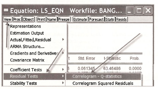
The EViews version of Figure 9.4 on page 241 of the text is obtained by first returning to the original least-squares estimated equation and selecting View/Residual Tests/Correlogram – Q statistics

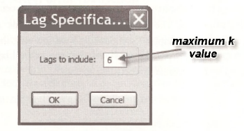
You will then be faced with the following Lag Specification window. Lags to include is the number of correlations r₁₅r₂,…,r_t that you would like EViews to calculate. In line with Figure 9.4, we choose 6. As we will see later in the chapter, larger numbers can be chosen when the sample size is larger.

Information on the r_k is presented in two ways. The numerical values appear in the column AC. A bar chart with each bar reflecting the magnitude and sign of each r_k is given in the column headed Autocorrelation. Bars long enough to obscure one of the dotted lines signify autocorrelations that are significantly different from zero at a 5% significance level.

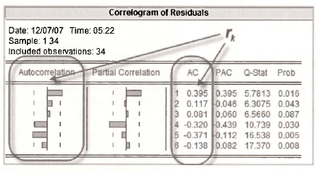
We will not be concerned with the remaining information. Partial Correlation (PAC), Q-Stat and their p-values, Prob, are covered in specialist time-series courses.

The orientation of the EViews graph is different to that of Figure 9.4, and the values of the correlations are slightly different, but the message is the same. The residual correlations for lags 1 and 5 are significantly different from zero at a 5% significance level. That at lag 4 is marginal.

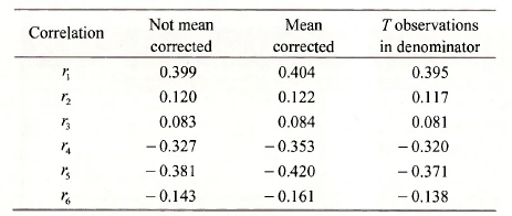
The correlations computed from the three alternative formulas are given in the table below. Those given on page 240 of the text correspond to those from the mean corrected formula.

After estimating the model assuming that the errors follow an AR( 1) model, one would hope that the new residuals, the v,, no longer exhibit autocorrelation. We can check them out by examining the residual correlogram from the estimated AR(1) error model. After opening the equation object for that model, and following the steps described above, we get the EViews version of Figure 9.5 on page 242 of the text.

No autocorrelations are clearly significantly different from zero at a 5% level, although those at lags 4 and 5 are marginal.

4.2. Lagrange multiplier (LM) test

In the context of the sugarcane example, the Lagrange multiplier test for an AR(1) error is a test of the significance of p, where p is the least squares estimate from either of the following two equations.

In both cases the e, are the least squares residuals. We will focus on the second equation. Both equations yield identical results for F- and t-tests on the significance of p. The second equation has the advantage of producing a further test value of the form LM = T x R². To obtain these values re-open the least squares estimated equation and select View/Residual Tests/Serial Correlation LM Test.

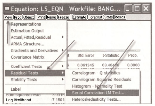
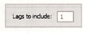
You will be asked how many lags to include. In this case we specify just 1. We are interested in testing for an AR(1) error and we only have one lag of e, on the right side of the equation. The correlogram was used to consider the general autocorrelation properties of the residuals.

The test results appear in the following output.

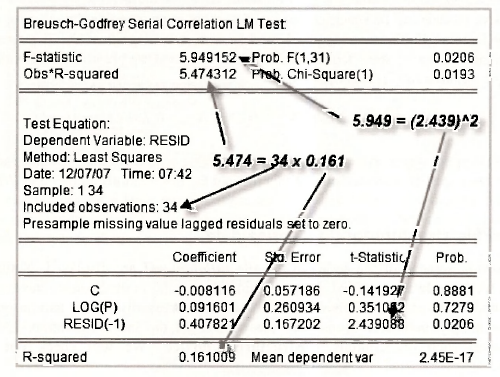
The two test values and their corresponding p-values are given at the top of the output. The value F = 5.949 is a test of the significance of p, the coefficient of RESID(-l) that appears in the bottom half of the output. Because F = 5.949 = t² = 2.439², the test can be performed as a t- or an F-test and the p-value of 0.0206 is the same in both cases. The other test is a x² – test with the test value being given by LM = T x R² = 34x 0.161 = 5.474 , and a p-value of 0.0193. In both cases a null hypothesis of H₀: p = 0 is rejected at a 5% significance level. Make sure that you can locate these various values on the output. And check them against p.242-3 of the text.

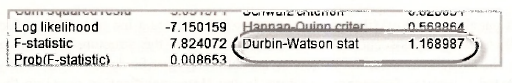
4.3. Durbin-Watson test

You may have noticed a Durbin-Watson value that is automatically provided on the least squares output. The Durbin Watson test is a test for AR(1) errors. It considered in Appendix 9B of the text. Its critical values and p-values are less readily computed than those for other tests for AR(1) errors, and so its popularity as a test is declining. Although EViews computes the value of the test statistic, it does not have commands for computing corresponding critical or p-values. As a rough guide, values of the Durbin-Watson statistic of 1.3 or less could be suggestive of autocorrelation. The value from the least-squares estimated sugarcane equation is 1.169.

5. AUTOREGRESSIVE MODELS

Autoregressive models can be specified not just for errors in an equation, but also for observable variables of interest. Furthermore, general models with more lags than the 1 assumed for the sugarcane example can be specified. In Section 9.5 of the text we are concerned with an AR(3) model for the inflation rate. It is given by

Data for inflation are stored in the file inflation.wfl, along with a number of other variables. Let us examine some special characteristics of this file and the observations on CPI. and INFLN.

5.1. Workfile structure for time series data

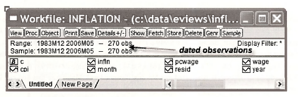
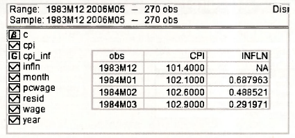
In the following screenshot the series in the file inflation.wfl are displayed. Notice how the Range and the Sample are specified. They contain dates. So far in the book we have mainly been concerned with cross-section observations which do not necessarily have a natural ordering and which were simply numbered from 1 to the number of the last observation. EViews calls workfiles with such observations Unstructured/Undated. We will check out the other alternatives.

To examine the workfile structure of the workfile inflation.wfl, select Proc/Structure/Resize Current Page.

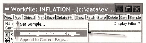
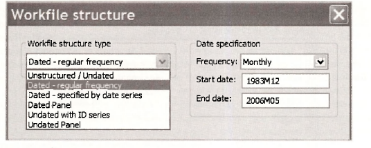
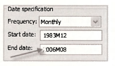
In the left panel of the Workfile structure window you can see a list of the Workfile structure types. When using cross-section data in earlier examples, the structure was Unstructured / Undated. Now we have moved on to time series data with specific dates for the observations, we use the Dated – regular frequency structure. In the Date specification panel on the right side the observations have been designated as Monthly in the Frequency box with 1983M12 (December, 1983) and 2006M05 (May, 2006) as the Start date and End date, respectively.

The other alternatives for a Date specification are illustrated below. The integer date option is used when specific dates have not been assigned to the observations. Such was the case with the Bangladesh sugarcane data that were simply allocated integer dates from 1 to 34.

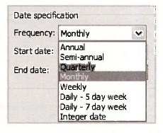
It should be kept in mind that the dating of observations is generally a convenience factor, not one that has a bearing on your results from estimation. As long as the sequence of the observations is the same it does not matter how you label them. Panel data situations that are dealt with later in the book are an exception. In this case it is important to set up the labeling to distinguish between time periods and cross sections, but providing this is done, the labeling of the time series observati ons does not matter. How to set up your workfile structure when reading data from another source is covered in Chapter 17.

5.2. Estimating AR models

Now that we have finished our short digression on workfile structure for time series data, we return to the AR(3) model for inflation. The first few observations in a spreadsheet for a group containing CPI and INFLN are given below, superimposed on the workfile window. There are 270 observations on CPI. The series INFLN has been generated using the command

series infln = (log(CPI) – log(CPI(-1)))*100

Because CPI(-1) is needed to compute INFLN, no observation on INFLN is available for the first observation in December, 1983. EViews records it as NA. That leaves 269 observations for estimating the AR(3) model. The need for values of INFLN , INFLN_t_₂ and INFLN_t₃ in the estimation process reduces the sample size for estimation by a further 3 to 266. This will become more apparent as we consider the results from estimation.

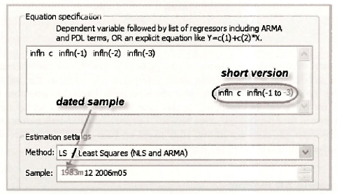
The AR model can be estimated using least squares and so estimation proceeds using the familiar EViews Equation specification window. The only new feature, but not something that is totally new, is how to specify the lagged variables INFLN_M, INFLN_t_₂ and INFLN_i_₃ as explanatory variables. We do that using the notation infln(-1), infln(-2) and infln(-3) as illustrated below. There is a shorter way of writing these three variables, however, one that is particularly useful if the number of lags is large. This short version is infln(-1 to -3). The only other difference at this stage is the nature of the Sample setting. In line with the workfile structure the sample is described in terms of the dates of the observations.

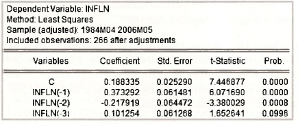
The output that appears matches that in equation (9.37) on page 245 of the text. Note again the way in which the sample is expressed and that it has been adjusted to accommodate the observations lost through lagging, leaving a total of 266.

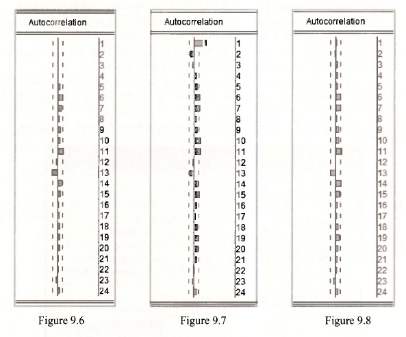
Ideally, the residuals from the estimated AR model should not exhibit any autocorrelation. This fact can be checked by examining the residual correlogram. After opening the equation object, select View/Residual Tests/Correlogram – Q statistics. Eviews will ask you for the number of lags to include. Choose 24, in line with Figure 9.6 on page 246 of the text. The correlogram, with a host of information, will appear. We are primarily interested in the autocorrelations and whether they are significantly different from zero. In the following screenshots we have isolated the bar charts of the correlations for Figures 9.6, 9.7 and 9.8. Relative to the figures in the text, the EViews bar charts are rotated 90 degrees. They have the lag on the “y-axis” and the correlations on the “x-axis”. Check the EViews version of Figure 9.6. We see that all correlations are very small, with those at lags 6, 11 and 13 marginally significant. Discussion of Figures 9.7 and 9.8 is deferred until later sections.

5.3. Forecasting with an AR model

The purpose of estimating the AR(3) model was to forecast inflation for the following 3 months, June, July and August of 2006. To make these forecasts we begin by extending the range of our workfile. Go back and have a quick re-read of Section 9.5.1. There you will see that we access the Workfile structure by selecting Proc/Structure/Resize Current Page. We change the End date of the Date specification to 2006M08 (August, 2006) and click OK. EViews will check whether you really want to make this change by asking Resize involves inserting 3 observations. Continue? Click Yes.

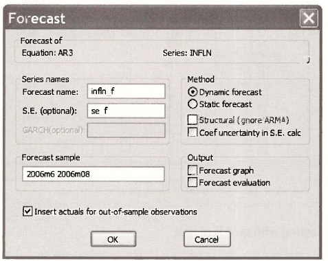
To compute the forecasts you fill in the Forecast dialog box that is obtained by opening the estimated equation, and then select Forecast. Several pieces of information are required.

We have assigned INFLN_F as the series name for the forecasts (Forecast name) and SE_F as the series name for the standard errors of the forecasts (S.E. (optional)).
The Forecast sample is June to August, 2006 that we specify as 2006m6 2006m8.
Ticking the box Insert actuals for out-of-sample observations means actual values for will be inserted in the series INFLN_F for the period 1983M12 to 2006M5.
Dynamic forecast is chosen for the Method because forecasts for future values will depend on earlier forecasts when actual values are not available.
Only error uncertainty, not coefficient uncertainty, is considered in the calculation of the forecast standard errors presented in Table 9.2 of the text and so the box Coef uncertainty in S.E. calc is not ticked.
We have not worried about Output for Forecast graph and Forecast evaluation.

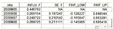
Clicking OK creates the series INFLN_F and SE_F. The relevant values are given in the last 3 rows of their respective spreadsheets. To complete the information in Table 9.2 of the text we need the upper and lower values for the 95% forecast intervals. These values can be created using the commands below. Ask yourself where the 262 comes from.

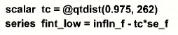
series fint_up = infln_f + tc*se_f

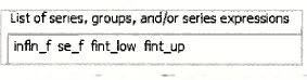
the values in Table 9.2 can be presented as follows.

6. FINITE DISTRIBUTED LAGS

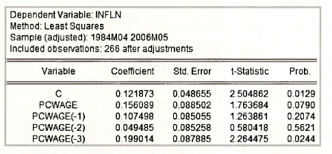
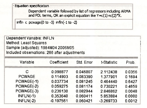
The finite distributed lag model in the text relates the inflation rate to current and past changes in the wage rate. The data are stored in the file inflation.wfl. The estimated model is

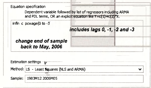
Note the shorthand notation for including all lags of PCWAGE. Also, remembering that we had extended the sample-for forecast-iag, yeu mad8«*ieed-to ehange the end of sample-back to 2006M05 for estimating this equation.

The results are those given in Table 9.3 of the text.

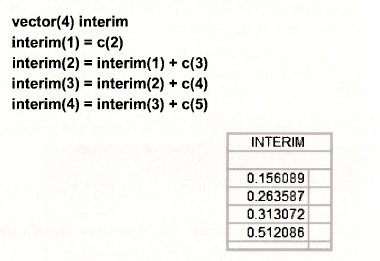
The delay multipliers in Table 9.4 are equal to the above coefficient estimates. The interim multipliers can be stored in a vector called INTERIM using the following commands.

Finally, we check the residual correlogram for evidence of autocorrelated residuals. Select View/Residual Tests/Correlogram – Q statistics. The autocorrelations from the resulting correlogram are presented back in Section 9.5.2, and entitled Figure 9.7. There is a significant autocorrelation at lag 1, and significant but smaller correlations at lags 6, 7, 10, 11 and 15.

7. AUTOREGRESSIVE DISTRIBUTED LAG MODELS

The ARDL model combines features of the AR model and the finite distributed lag model. Its estimation does not require any EViews commands or options that we have not already covered. Thus, this section is one where we revise and consolidate material from earlier parts of the chapter. The model to be estimated is

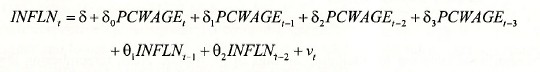
The corresponding equation specification and results follow. See page 251 of the text.

The autocorrelations from the residual correlogram are presented back in Section 9.5.2, and entitled Figure 9.8. There are significant but very small autocorrelations at lags 6, 7, 11, 13 and 14.

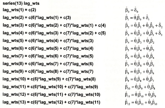
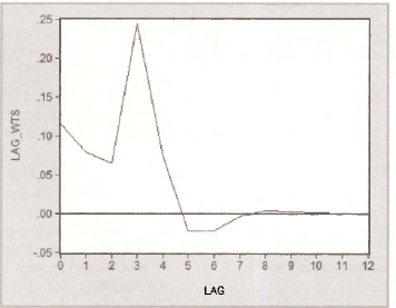
7.1. Graphing the lag weights

The lag weights that are graphed in Figure 9.9 can be obtained recursively using the commands below. As you can see, calculating them individually as we have done is an unrewarding repetitive task. It can be avoided by programming a do loop, something that you will learn as you study more econometrics and start using the lull version of EViews.

To create the graph in Figure 9.9 we also need a series called LAG. A command that produces this series is

series lag = @trend

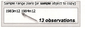
The EViews function @trend defines a trend series beginning at zero and with each observation incremented by 1, giving the values 0,1, 2,… Now, since there are only 13 values to graph, we need to restrict the sample to the first 13 observations. The monthly dates EViews has attached to its sample observations are not really relevant in this case, but we can trick EViews by cutting the sample back to the first 13 months. Select Sample from the workfile window and insert the following start and end dates.

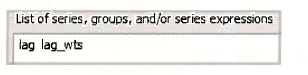
Then select Object/New Object/Graph. Name it FIGURE9_9. Enter the two series for the graph, with the one on the x-axis first.

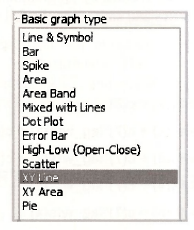
The graph FIGURE9_9 will appear in your workfile. However, it will need a bit of work before it is presentable. To ensure it is of the correct type, go to Options/Type/XY Line. Click Apply.

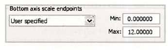
To make the x-axis compatible with Figure 9.9, go to Axis/Scale/Edit Axis/Bottom Axis and Scale. Then, for Bottom axis scale endpoints, choose User specified and specify 0 as the Min and 12 as the Max. Click Apply. Click OK.

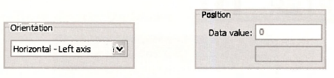
To draw a horizontal line at 0, go to Line/Shade, select Line for Type. Choose Orientation and specify the Data value as follows.

Voila! A respectable looking Figure 9.9 appears.

Source: Griffiths William E., Hill R. Carter, Lim Mark Andrew (2008), Using EViews for Principles of Econometrics, John Wiley & Sons; 3rd Edition.