When you use discounted cash flow (DCF) to value a project, you implicitly assume that the firm will hold the assets passively. But managers are not paid to be dummies. After they have invested in a new project, they do not simply sit back and watch the future unfold. If things go well, the project may be expanded; if they go badly, the project may be cut back or abandoned altogether. Projects that can be modified in these ways are more valuable than those that do not provide such flexibility. The more uncertain the outlook, the more valuable this flexibility becomes.
That sounds obvious, but notice that sensitivity analysis and Monte Carlo simulation do not recognize the opportunity to modify projects.[1] For example, think back to the Otobai electric scooter project. In real life, if things go wrong with the project, Otobai would abandon to cut its losses. If so, the worst outcomes would not be as devastating as our sensitivity analysis and simulation suggested.
Options to modify projects are known as real options. Managers may not always use the term “real option” to describe these opportunities; for example, they may refer to “intangible advantages” of easy-to-modify projects. But when they review major investment proposals, these option intangibles are often the key to their decisions.
1. The Option to Expand
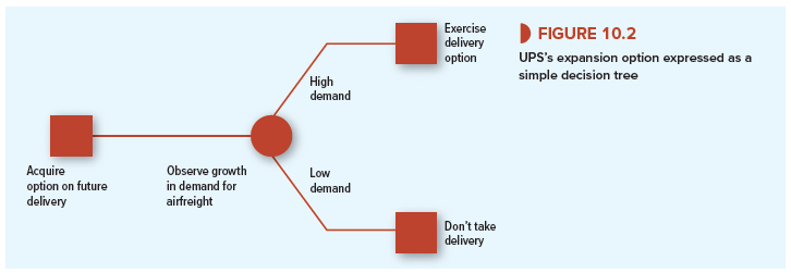
Long-haul airfreight businesses such as UPS need to move a massive amount of goods each day. To handle the growing demand, UPS announced in 2016 that it had agreed to buy 14 Boeing freighter aircraft to add to its existing fleet of more than 500 planes. If business continued to expand, UPS would need more aircraft. But rather than placing additional firm orders, the company secured a place in Boeing’s production line by acquiring options to buy a further 14 aircraft at a predetermined price. These options did not commit UPS to expand but gave it the flexibility to do so.
Figure 10.2 displays UPS’s expansion option as a simple decision tree. You can think of it as a game between UPS and fate. Each square represents an action or decision by the company. Each circle represents an outcome revealed by fate. In this case, there is only one outcome— when fate reveals the airfreight demand and UPS’s capacity needs. UPS then decides whether to exercise its options and buy the additional aircraft. Here the future decision is easy: Buy the airplanes only if demand is high and the company can operate them profitably. If demand is low, UPS walks away and leaves Boeing with the problem of finding another customer for the planes that were reserved for UPS.
You can probably think of many other investments that take on added value because of the further options they provide. For example,
- When launching a new product, companies often start with a pilot program to iron out possible design problems and to test the market. The company can evaluate the pilot project and then decide whether to expand to full-scale production.
- When designing a factory, it can make sense to provide extra land or floor space to reduce the future cost of a second production line.
- When building a four-lane highway, it may pay to build six-lane bridges so that the road can be converted later to six lanes if traffic volumes turn out to be higher than expected.
- When building production platforms for offshore oil and gas fields, companies usually allow ample vacant deck space. The vacant space costs more up front but reduces the cost of installing extra equipment later. For example, vacant deck space could provide an option to install water-flooding equipment if oil or gas prices are high enough to justify this investment.
Expansion options do not show up on accounting balance sheets, but managers and investors are well aware of their importance. For example, in Chapter 4 we showed how the present value of growth opportunities (PVGO) contributes to the value of a company’s common stock. PVGO equals the forecasted total NPV of future investments. But it is better to think of PVGO as the value of the firm’s options to invest and expand. The firm is not obliged to grow. It can invest more if the number of positive-NPV projects turns out high, or it can slow down if that number turns out low. The flexibility to adapt investment to future opportunities is one of the factors that makes PVGO so valuable.
2. The Option to Abandon
If the option to expand has value, what about the decision to bail out? Projects do not just go on until assets expire of old age. The decision to terminate a project is usually taken by management, not by nature. Once the project is no longer profitable, the company will cut its losses and exercise its option to abandon the project.
Some assets are easier to bail out of than others. Tangible assets are usually easier to sell than intangible ones. It helps to have active secondhand markets, which exist mainly for standardized items. Real estate, airplanes, trucks, and certain machine tools are likely to be relatively easy to sell. On the other hand, the knowledge accumulated by a software company’s research and development program is a specialized intangible asset and probably would not have significant abandonment value. (Some assets, such as old mattresses, even have negative abandonment value; you have to pay to get rid of them. It is costly to decommission nuclear power plants or to reclaim land that has been strip-mined.)
Example 10.1 • Bailing Out of the Outboard-Engine Project
Managers should recognize the option to abandon when they make the initial investment in a new project or venture. For example, suppose you must choose between two technologies for production of a Wankel-engine outboard motor.
- Technology A uses computer-controlled machinery custom-designed to produce the complex shapes required for Wankel engines in high volumes and at low cost. But if the Wankel outboard does not sell, this equipment will be worthless.
- Technology B uses standard machine tools. Labor costs are much higher, but the machinery can be sold for $17 million if demand turns out to be low.
Just for simplicity, assume that the initial capital outlays are the same for both technologies. If demand in the first year is buoyant, technology A will provide a payoff of $24 million. If demand is sluggish, the payoff from A is $16 million. Think of these payoffs as the project’s
cash flow in the first year of production plus the value in year 1 of all future cash flows. The corresponding payoffs to technology B are $22.5 million and $15 million:
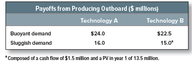
Technology A looks better in a DCF analysis of the new product because it was designed to have the lowest possible cost at the planned production volume. Yet you can sense the advantage of the flexibility provided by technology B if you are unsure whether the new outboard will sink or swim in the marketplace. If you adopt technology B and the outboard is not a success, you are better off collecting the first year’s cash flow of $1.5 million and then selling the plant and equipment for $17 million.
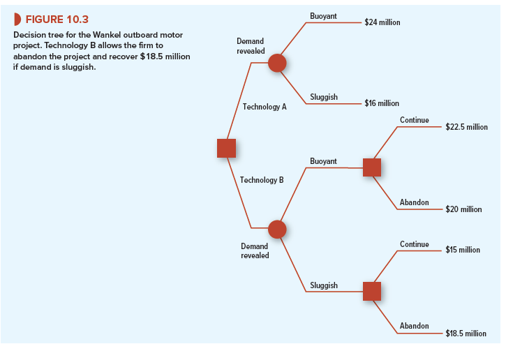
Figure 10.3 summarizes Example 10.1 as a decision tree. The abandonment option occurs at the right-hand boxes for technology B. The decisions are obvious: Continue if demand is buoyant, abandon otherwise. Thus the payoffs to technology B are
Buoyant demand → continue production → payoff of $22.5 million
Sluggish demand → exercise option to sell assets → payoff of 1.5 + 17 = $18.5 million
Technology B provides an insurance policy: If the outboard’s sales are disappointing, you can abandon the project and receive $18.5 million. The total value of the project with technology B is its DCF value, assuming that the company does not abandon, plus the value of the option to sell the assets for $17 million. When you value this abandonment option, you are placing a value on flexibility.
3. Production Options
When companies undertake new investments, they generally think about the possibility that they may wish to modify the project at a later stage. After all, today everybody may be demanding round pegs, but, who knows, tomorrow square ones may be all the rage. In that case, you need a plant that provides the flexibility to produce a variety of peg shapes. In just the same way, it may be worth paying up front for the flexibility to vary the inputs. For example, in Chapter 22, we will describe how electric utilities often build in the option to switch between burning oil and burning natural gas. We refer to these opportunities as production options.
4. Timing Options
The fact that a project has a positive NPV does not mean that it is best undertaken now. It might be even more valuable to delay.
Timing decisions are fairly straightforward under conditions of certainty. You need to examine alternative dates for making the investment and calculate its net future value at each of these dates. Then, to find which of the alternatives would add most to the firm’s current value, you must discount these net future values back to the present:
![]()
The optimal date to undertake the investment is the one that maximizes its contribution to the value of your firm today. This procedure should already be familiar to you from Chapter 6, where we worked out when it was best to cut a tract of timber.
In the timber-cutting example, we assumed that there was no uncertainty about the cash flows, so that you knew the optimal time to exercise your option. When there is uncertainty, the timing option is much more complicated. An investment opportunity not taken at t = 0 might be more or less attractive at t = 1; there is rarely any way of knowing for sure. Perhaps it is better to strike while the iron is hot even if there is a chance that it will become hotter. On the other hand, if you wait a bit you might obtain more information and avoid a bad mistake. That is why you often find that managers choose not to invest today in projects where the NPV is only marginally positive and there is much to be learned by delay.
5. More on Decision Trees
We will return to all these real options in Chapter 22, after we have covered the theory of option valuation in Chapters 20 and 21. But we will end this chapter with a closer look at decision trees.
Decision trees are commonly used to describe the real options imbedded in capital investment projects. But decision trees were used in the analysis of projects years before real options were first explicitly identified. Decision trees can help to illustrate project risk and how future decisions will affect project cash flows. Even if you never learn or use option valuation theory, decision trees belong in your financial toolkit.
The best way to appreciate how decision trees can be used in project analysis is to work through a detailed example.
Example 10.2 • A Decision Tree for Pharmaceutical R&D
Drug development programs may last decades. Usually hundreds of thousands of compounds may be tested to find a few with promise. Then these compounds must survive several stages of investment and testing to gain approval from the Food and Drug Administration (FDA). Only then can the drug be sold commercially. The stages are as follows:
- Phase I clinical trials. After laboratory and clinical tests are concluded, the new drug is tested for safety and dosage in a small sample of humans.
- Phase II clinical trials. The new drug is tested for efficacy (Does it work as predicted?) and for potentially harmful side effects.
- Phase III clinical trials. The new drug is tested on a larger sample of humans to confirm efficacy and to rule out harmful side effects.
- Prelaunch. If FDA approval is gained, there is investment in production facilities and initial marketing. Some clinical trials continue.
- Commercial launch. After making a heavy initial investment in marketing and sales, the company begins to sell the new drug to the public.
Once a drug is launched successfully, sales usually continue for about 10 years, until the drug’s patent protection expires and competitors enter with generic versions of the same chemical compound. The drug may continue to be sold off-patent, but sales volume and profits are much lower.
The commercial success of FDA-approved drugs varies enormously. The PV of a “blockbuster” drug at launch can be 5 or 10 times the PV of an average drug. A few blockbusters can generate most of a large pharmaceutical company’s profits.[2]
No company hesitates to invest in R&D for a drug that it knows will be a blockbuster. But the company will not find out for sure until after launch. Occasionally, a company thinks it has a blockbuster only to discover that a competitor has launched a better drug first.
Sometimes the FDA approves a drug but limits its scope of use. Some drugs, though effective, can only be prescribed for limited classes of patients; other drugs can be prescribed much more widely. Thus the manager of a pharmaceutical R&D program has to assess the odds of clinical success and the odds of commercial success. A new drug may be abandoned if it fails clinical trials—for example, because of dangerous side effects—or if the outlook for profits is discouraging.
Figure 10.4 is a decision tree that illustrates these decisions. We have assumed that a new drug has passed phase I clinical trials with flying colors. Now it requires an investment of $18 million for phase II trials. These trials take two years. The probability of success is 44%.
If the trials are successful, the manager learns the commercial potential of the drug, which depends on how widely it can be used. Suppose that the forecasted PV at launch depends on the scope of use allowed by the FDA. These PVs are shown at the far right of the decision tree: an upside outcome of NPV = $700 million if the drug can be widely used, a most likely case with NPV = $300 million, and a downside case of NPV = $100 million if the drug’s scope is greatly restricted.[3] The NPVs are the payoffs at launch after investment in marketing. Launch comes three years after the start of phase III if the drug is approved by the FDA.
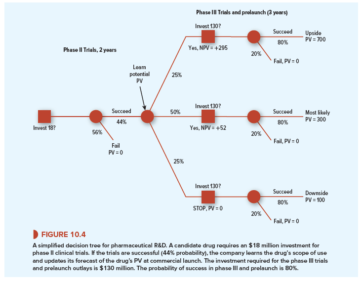
The probabilities of the upside, most likely, and downside outcomes are 25%, 50%, and 25%, respectively.
A further R&D investment of $130 million is required for phase III trials and for the prelaunch period. (We have combined phase III and prelaunch for simplicity.) The probability of FDA approval and launch is 80%.
Now let’s value the investments in Figure 10.4. We assume a risk-free rate of 4% and market risk premium of 7%. If FDA-approved pharmaceutical products have asset betas of .8, the opportunity cost of capital is 4 + .8 X 7 = 9.6%.
We work back through the tree from right to left. The NPVs at the start of phase III trials are:
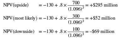
Since the downside NPV is negative at -$69 million, the $130 million investment at the start of phase III should not be made in the downside case. There is no point investing $130 million for an 80% chance of a $100 million payoff three years later. Therefore the value of the R&D program at this point in the decision tree is not -$69 million, but zero.
Now calculate the NPV at the initial investment decision for phase II trials. The payoff two years later depends on whether the drug delivers on the upside, most likely, or downside: a 25% chance of NPV = +$295 million, a 50% chance of NPV = +$52 million, and a 25% chance of cancellation and NPV = 0. These NPVs are achieved only if the phase II trials are successful: There is a 44% chance of success and a 56% chance of failure. The initial investment is $18 million. Therefore, NPV is
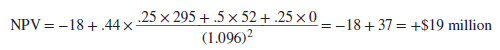
Thus the phase II R&D is a worthwhile investment, even though the drug has only a 33% chance of making it to launch (.44 x .75 = .33, or 33%).
Notice that we did not increase the 9.6% discount rate to offset the risks of failure in clinical trials or the risk that the drug will fail to generate profits. Concerns about the drug’s efficacy, possible side effects, and scope of use are diversifiable risks, which do not increase the risk of the R&D project to the company’s diversified stockholders. We were careful to take these concerns into account in the cash-flow forecasts, however. The decision tree in Figure 10.4 keeps track of the probabilities of success or failure and the probabilities of upside and downside outcomes.10
Figures 10.3 and 10.4 are both examples of abandonment options. We have not explicitly modeled the investments as options, however, so our NPV calculation is incomplete. We show how to value abandonment options in Chapter 22.
6. Pro and Con Decision Trees
Any cash-flow forecast rests on some assumption about the firm’s future investment and operating strategy. Often that assumption is implicit. Decision trees force the underlying strategy into the open. By displaying the links between today’s decisions and tomorrow’s decisions, they help the financial manager to find the strategy with the highest net present value.
The decision tree in Figure 10.4 is a simplified version of reality. For example, you could expand the tree to include a wider range of NPVs at launch, possibly including some chance of a blockbuster or of intermediate outcomes. You could allow information about the NPVs to arrive gradually, rather than just at the start of phase III. You could introduce the investment decision at phase I trials and separate the phase III and prelaunch stages. You may wish to draw a new decision tree covering these events and decisions. You will see how fast the circles, squares, and branches accumulate.
The trouble with decision trees is that they get so_complex so_quickly (insert your own expletives). Life is complex, however, and there is very little we can do about it. It is therefore unfair to criticize decision trees because they can become complex. Our criticism is reserved for analysts who let the complexity become overwhelming. The point of decision trees is to allow explicit analysis of possible future events and decisions. They should be judged not on their comprehensiveness but on whether they show the most important links between today’s and tomorrow’s decisions. Decision trees used in real life will be more complex than Figure 10.4, but they will nevertheless display only a small fraction of possible future events and decisions. Decision trees are like grapevines: They are productive only if they are vigorously pruned.
Wow, wonderful blog layout! How long have you been blogging for? you made blogging look easy. The overall look of your website is magnificent, let alone the content!