Sensitivity analysis allows you to consider the effect of changing one variable at a time. By looking at the project under alternative scenarios, you can consider the effect of a limited number of plausible combinations of variables. Monte Carlo simulation is a tool for considering all possible combinations. It therefore enables you to inspect the entire distribution of project outcomes.
Imagine that you are a gambler at Monte Carlo. You know nothing about the laws of probability (few casual gamblers do), but a friend has suggested to you a complicated strategy for playing roulette. Your friend has not actually tested the strategy but is confident that it will on the average give you a 2.5% return for every 50 spins of the wheel. Your friend’s optimistic estimate for any series of 50 spins is a profit of 55%; your friend’s pessimistic estimate is a loss of 50%. How can you find out whether these really are the odds? An easy but possibly expensive way is to start playing and record the outcome at the end of each series of 50 spins. After, say, 100 series of 50 spins each, plot a frequency distribution of the outcomes and calculate the average and upper and lower limits. If things look good, you can then get down to some serious gambling.
An alternative is to tell a computer to simulate the roulette wheel and the strategy. In other words, you could instruct the computer to draw numbers out of its digital hat to determine the outcome of each spin of the wheel and then to calculate how much you would make or lose from the particular gambling strategy.
That would be an example of Monte Carlo simulation. In capital budgeting, we replace the gambling strategy with a model of the project and the roulette wheel with a model of the world in which the project operates. Let us see how this might work with our project for an electrically powered scooter.
1. Simulating the Electric Scooter Project
Step 1: Modeling the Project The first step in any simulation is to give the computer a precise model of the project. For example, the sensitivity analysis of the scooter project was based on the following implicit model of each year’s cash flow:
Cash flow = operating cash flow – investment in working capital
Operating cash flow = (revenue – costs – depreciation) x (1 – tax rate) + depreciation Revenue
= unit sales x unit price
Costs = (revenue x variable cost as a proportion of revenue) + fixed cost
This model of the project was all that you needed for the simpleminded sensitivity analysis that we described above. But if you wish to simulate the whole project, you need to think about how the variables are interrelated. For example, consider the unit sales variable. The marketing department has estimated sales of 6.8 million scooters in the first year of the project’s life; of course, you do not know how things will work out. Actual sales will exceed or fall short of expectations by the amount of the department’s forecast error:
Sales, year 1 = expected sales, year 1 x (1 + forecast error, year 1)
You expect the forecast error to be zero, but it could turn out to be positive or negative. Suppose, for example, that actual sales turn out to be 7.48 million. That means a forecast error of 10%, or +.1:
Sales, year 1 = 6.8 x (1 + .1) = 7.48 million
You can write sales in the second year in exactly the same way:
Sales, year 2 = expected sales, year 2 x (1 + forecast error, year 2)
At this point, you must consider how the expected sales in year 2 are affected by what happens in year 1. If scooter sales are below expectations in year 1, it is likely that they will continue to be below in subsequent years. Suppose that a shortfall in year 1 leads you to revise down your forecast of sales in year 2 by a like amount. Then:
Expected sales, year 2 = actual sales, year 1
Now you can rewrite sales in year 2 in terms of the actual sales in the previous year plus a forecast error:
Sales, year 2 = sales, year 1 x (1 + forecast error, year 2)
In the same way, you can describe the expected sales in year 3 in terms of sales in year 2 and so on. This set of equations illustrates how you can describe interdependence between different periods. But you also need to allow for interdependence between different variables. For example, if sales are high, the price of electrically powered scooters is likely to be above forecast. Suppose that this is the only uncertainty and that a 10% addition to sales would lead you to predict a 3% increase in price. Then you could model the first year’s price as follows:
Price, year 1 = expected price, year 1 x (1 + .3 x error in sales forecast, year 1)
Then, if variations in sales exert a permanent effect on price, you can define the second year’s price as
Price, year 2 = expected price, year 2 x (1 + .3 x error in sales forecast, year 2)
= actual price, year 1 x (1 + .3 x error in sales forecast, year 2)
Notice how we have linked each period’s selling price to the actual selling prices (including forecast error) in all previous periods. We used the same type of linkage for sales. These linkages mean that forecast errors accumulate; they do not cancel out over time. Thus, uncertainty increases with time: The farther out you look into the future, the more the actual price or sales may depart from your original forecast. The complete model of your project would include a set of equations for each of the variables: sales, price, variable cost, fixed cost, and investment in working capital. Even if you allowed for only a few interdependencies between variables and across time, the result would be quite a complex list of equations. Perhaps that is not a bad thing if it forces you to understand what the project is all about. Model building is like spinach: You may not like the taste, but it is good for you.
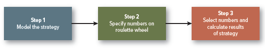
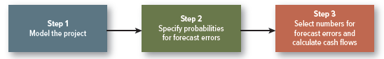
Step 2: Specifying Probabilities Remember the procedure for simulating the gambling strategy? The first step was to specify the strategy, the second was to specify the numbers on the roulette wheel, and the third was to tell the computer to select these numbers at random and calculate the results of the strategy:
The steps are just the same for your scooter project:
Think about how you might go about specifying your possible errors in forecasting market size. You expect sales in year 1 to be 6.8 million scooters. You obviously don’t think you are underestimating or overestimating, so the expected forecast error is zero. On the other hand, the marketing department has given you a range of possible estimates. Sales in year 1 could be as low as 5.7 million scooters or as high as 8.2 million scooters. Thus the forecast error has an expected value of 0 and a range of plus or minus 20%. If the marketing department has, in fact, given you the lowest and highest possible outcomes, actual market size should fall somewhere within this range with near certainty.[1]
That takes care of market size; now you need to draw up similar estimates of the possible forecast errors for each of the other variables that are in your model.
Step 3: Simulate the Cash Flows The computer now samples from the distribution of the forecast errors, calculates the resulting cash flows for each period, and records them. After many iterations, you begin to get accurate estimates of the probability distributions of the project cash flows—accurate, that is, only to the extent that your model and the probability distributions of the forecast errors are accurate. Remember the GIGO principle: “garbage in, garbage out.”
Step 4: Calculate Present Value The distributions of project cash flows should allow you to calculate the expected cash flows more accurately. In the final step, you need to discount these expected cash flows to find present value.
Simulation, though complicated, has the obvious merit of compelling the forecaster to face up to uncertainty and to interdependencies. Once you have set up your simulation model, it is a simple matter to analyze the principal sources of uncertainty in the cash flows and to see how much you could reduce this uncertainty by improving the forecasts of sales or costs. You may also be able to explore the effect of possible modifications to the project.
Simulation may sound like a panacea for the world’s ills, but, as usual, you pay for what you get. Sometimes you pay for more than you get. It is not just a matter of the time spent in building the model. It is extremely difficult to estimate interrelationships between variables and the underlying probability distributions, even when you are trying to be honest. But in capital budgeting, forecasters are seldom completely impartial and the probability distributions on which simulations are based can be highly biased.
In practice, a simulation that attempts to be realistic will also be complex. Therefore, the decision maker may delegate the task of constructing the model to management scientists or consultants. The danger here is that even if the builders understand their creation, the decision maker cannot and therefore does not rely on it. This is a common but ironic experience.
Good info. Lucky me I reach on your website by accident, I bookmarked it.