The Multiple Linear Regression Model by using EViews

In the simple linear regression model the average value of a dependent variable is modeled as a linear function of a constant and a single explanatory variable. The multiple linear regression model expands the number of explanatory variables. As such it is a simple but important extension that makes linear regression quite powerful.

The example used in this chapter is a model of sales for Big Andy’s Burger Barn. Big Andy’s sales revenue depends on the prices charged for hamburgers, fries, shakes, and so on, and on the level of advertising. The prices charged in a given city are collected together into a weighted price index that is denoted by P = PRICE and measured in dollars. Monthly sales revenue for a given city is denoted by S = SALES and measured in $1,000 units. Advertising expenditure for each city A = ADVERT is also measured in thousands of dollars. The model includes two explanatory variables and a constant and is written as

SALES = E(SALES) + e = β₁ + β₂PRICE + β₃ ADVERT + e

In this Chapter we use EViews to estimate this model, to obtain forecasts from the model, to examine the covariance matrix and standard errors of the estimates, and to compute confidence intervals and hypothesis test values for each of the coefficients. While performing these tasks we reinforce some of the EViews steps described in earlier chapters as well as introduce some new ones.

1. THE WORKFILE: SOME PRELIMINARIES

Observations on SALES, PRICE and ADVERT for 75 cities are available in the file andy.wfl. Opening this file as described in Chapters 1 and 2 yields the following screen

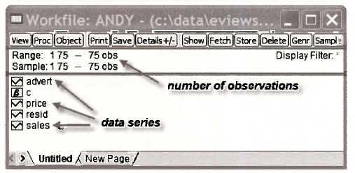
Note that the range and sample are set at 75 observations. And note the location of the data series in the workfile. The other objects C and RESID appear automatically in all EViews workfiles. We explain them as they become needed.

1.1. Naming the page

It is possible to use a number of “pages” within the same EViews file. We will rarely use this option because most problems can fit neatly within the one page. However, if working with an untitled page is disconcerting for you, you can give it a name by selecting from your workfile toolbar Proc/Rename Current Page

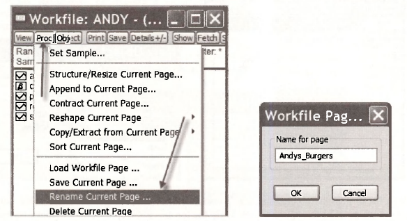
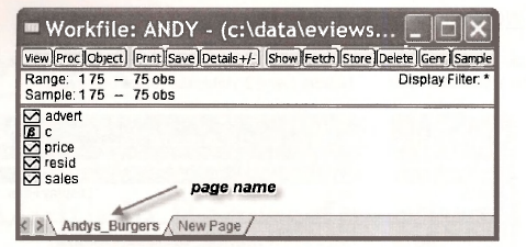
A window appears in which you can name the page. After choosing the name Andys_Burgers, your workfile will appear as

1.2. Creating objects: a group

The data on each of the variables SALES., PRICE and ADVERT can be examined one at a time or as a group, as described in Chapters 1 and 2. We will create a group and then check the data and summary statistics to make sure they match those in Table 5.1 on page 109 of the text. In Chapters 1 and 2 we created a group by (1) highlighting the series to be included in the group, (2) double clicking the highlighted area, and (3) selecting Open Group. To extend your knowledge of EViews, we now describe another way. This new way is more cumbersome, but it will help you understand the more general concept of an object and how objects are created.

A group is one of many types of objects that can be created by EViews. The concept of an object is a bit vague, but you can think of it as anything that gets stored in your workfile. As Richard Startz says in EViews Illustrated [QMS, 2007, p.5], “object is a computer science buzz word meaning ‘thingie’.” Several chapters of the Startz book can be found under Help.

To see a list of possible objects, select Object/New Object from the workfile toolbar.

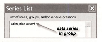
A long list of possible objects appears. We will encounter many of these objects (but not all of them) as we proceed through the book. Only the top few are displayed in the above screen shot. At present we select Group as the relevant object, and then click OK. We have left Name for object as Untitled. We will name it later. In the following window that appears, we type the names of the series to be included in the group, and then click OK.

The following screen appears. Note that the first 5 observations are the same as those in Table 5.1 on page 109 of the text. The last 3 observations can be checked by scrolling down.

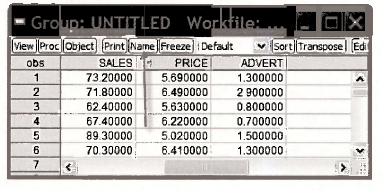
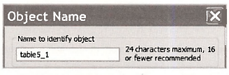
By selecting Name we can name the group object in the following window. In line with the text, we call it table5 1.

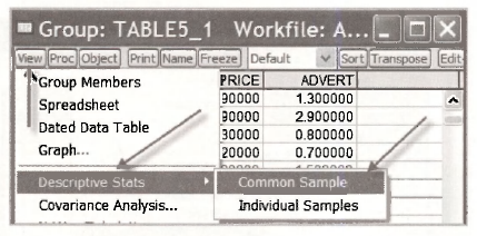
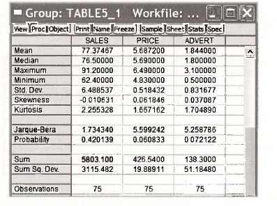
One of the advantages of creating a group of variables is that we can view a variety of information on the collection of variables in that group. The list of observations that we checked against Table 5.1 is one type of information; it is called the spreadsheet view of the group. Another useful view is the Descriptive Stats view that gives summary statistics that can be checked against those that appear in the lower panel of Table 5.1. To obtain this view we open the group and then select View/Descriptive Stats/Common Sample.

The summary statistics appear in the following window. In addition to the sample mean, median, maximum, minimum and standard deviation for each series, the table presents skewness and
kurtosis measures (see pages 490, 511 and 512 of the text), the value of the Jarque-Bera statistic for testing whether a series is normally distributed and its corresponding p-value (see pages 89-90 of the text), and the sum ∑x and sum of squared deviations ∑(x,-x)² for each of the series. Stop and check to see if you know how to obtain the standard deviation values from the sum of squared deviations.

2. ESTIMATING A MULTIPLE REGRESSION MODEL

The steps for estimating a multiple regression model are a natural extension of those for estimating a simple regression. We will consider two alternative ways. One is using the Quick menu considered in earlier chapters. The other is via the Object menu that we used in the previous section to define a group.

2.1. Using the Quick menu

To use the Quick menu for estimating an equation go to the upper EViews window and select Quick/Estimate Equation.

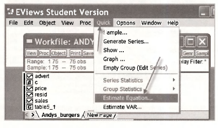
An Equation Estimation window appears. We add to it in the following way.

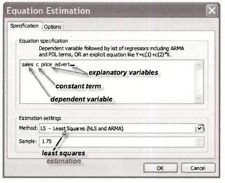
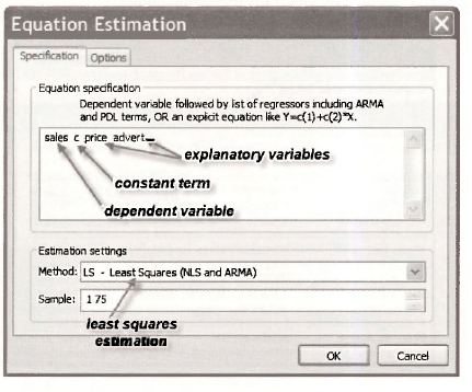
The Equation Specification dialog box is where you tell EViews what model you would like to estimate. Our equation is

SALES =  β₁ + β₂PRICE + β₃ ADVERT + e

The dependent variable SALES is inserted first, followed by the constant C and the explanatory variables PRICE and ADVERT. Under Estimation settings in the lower half of the window, you can choose the estimation Method and the Sample observations to be used for estimation. The least-squares method is the one we want, and the one that is automatically used unless another one is selected. A sample of 1 75 means that all observations in our sample are being used to estimate the equation. Clicking OK yields the regression output.

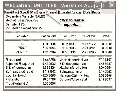
Compare this output with Table 5.2 on page 112 of the text. Least squares estimates of the coefficients β_1, β₂ and β₃ appear in the column Coefficient; their standard errors are in the column Std. Error; t-values for testing a zero null hypothesis for each of the coefficients appear in the column t-Statistic; and p-values for two-tail versions of these tests are given in the column Prob. From the bottom panel in the output, make sure you can locate R² = 0.4483, σ_y = 6.4885, SSE – ∑e² =1718.943 and the estimated standard deviation of the error term σ = 4.8861. Also, you should make sure you know how to compute (a) a from the value of SSE (page 114 of the text), and (b) R² from SSE and σ_v (page 125 of the text).

2.2. Using the Object menu

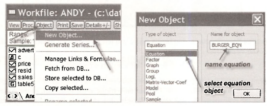
The same results can be obtained by direct creation of the relevant equation object. To proceed in this way select Object/New Object from the workfile toolbar. In the resulting New Object window, select Equation as the Type of object. Then, name the object (we chose BURGER EQN) and click OK.

The Equation Estimation window will appear. It can be filled in as described earlier.

Clicking OK yields the same regression output that we illustrated earlier using the quick menu.

After closing the output window, check the EViews workfile and note that, since you opened the workfile, two new objects have been added. These objects are the group of variables TABLE5_1 and the estimated equation BURGER_EQN. To reopen one of these objects, highlight it, and then double click.

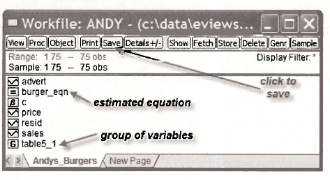
To ensure the estimated equation and the group of variables are retained for future use, click save. If you wish to save the file under another name so that the original workfile with data only is preserved, go to the upper EViews toolbar and select File/Save As.

3. FORECASTING FROM A REGRESSION MODEL

How to use EViews to obtain forecasts was considered extensively in Chapter 4 for both linear and log-linear models. Those procedures carry over directly to the multiple regression model. In this section we reinforce those procedures by showing how EViews can be used to forecast (or predict) hamburger sales revenue for PRICE -5.5 and ADVERT = 1.2, as is done on page 113 of the text. Two preliminary explanatory remarks are in order. First, note that we are using the terms “forecast” and “predict” interchangeably; each one has no special significance. Second, the steps we follow do not mimic exactly those in Chapter 4. The variations are deliberate. They are designed to expose you to more of the features of EViews. As in Chapter 4, we consider a simple forecasting procedure and one using EViews special forecasting capabilities. While the simple one is ideal for obtaining a single static forecast, it is not convenient for obtaining a forecast standard error, and it less than ideal for dynamic forecasting, a topic considered in Chapter 9.

3.1. A simple forecasting procedure

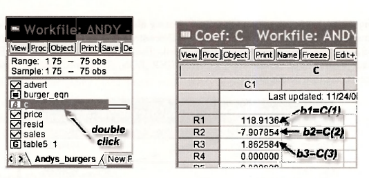
After you use EViews to estimate a regression model the estimated coefficients are stored in the object C that appears in your workfile. You can check this fact out by highlighting C and double clicking it. A spreadsheet will appear with the estimates stored in a column called Cl. In further commands that you might supply to EViews, the three values in that column can be used by referring to them as C(l), C(2) and C(3), respectively. That is, in terms of notation used in the book, the least squares estimates are

b₁=C(1)       b₂=C( 2)        b₃=C( 3)

Our objective is to get EViews to perform the calculation

The corresponding EViews command is

scalar sales_f = c(1) + c(2)*5.5 + c(3)*1.2

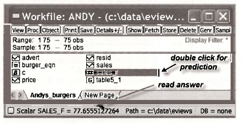
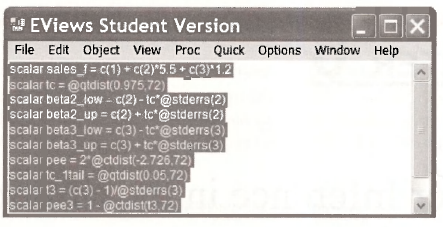
The first word scalar tells EViews that we are computing a scalar object (a single number) to be stored in the workfile. The second word sales_f is the name we are giving to that scalar object which is our predicted value. The right side of the equation performs the calculation. The command is placed in the upper EViews window as shown below.

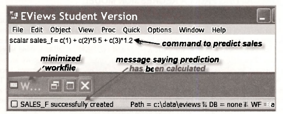
This window might look a little strange to you. We have compressed the typical EViews window so that we can show you all the information in a convenient space. The workfile has been temporarily minimized to move it out of the way. Then the bottom of the window has been moved upwards. Notice two things. The command to predict sales has been typed in the upper window. And, there is a message at the bottom indicating that the scalar object SALES_F has been successfully calculated. Providing you have not done something wrong that offends EViews, this message will appear after you type in the command and push the enter key.

A word of warning: The values C(l), C(2) and C(3) will always be the coefficient estimates for the model most recently estimated. If you have only estimated one equation, there will be no confusion. However, if you have estimated another model, successfully or not, the values will change. Make sure you are using the correct ones.

You have now calculated the forecast. How do you read off the answer? Go to the SALES_F object in your workfile and double click it. The answer appears in the bottom panel of your workfile.

3.2. Using the forecast option

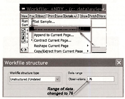
To use EViews automatic forecast command to produce out-of-sample forecasts, it is necessary to extend the size of the workfile to accommodate the observations for which we want forecasts. To do so you select, from the workfile toolbar, Proc/Structure/Resize Current Page. In this case, since we are only forecasting for one extra observation, we change the range from 75 to 76.

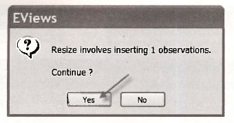
EViews will ask you whether you are sure you wish to make this change.

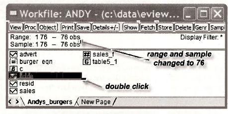
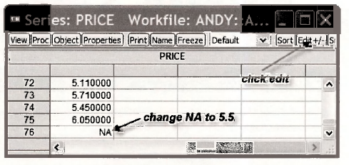
Notice that both the range and the sample in the workfile have changed from 1 75 to 1 76. The next task is the insert the values PRICE = 5.5 and ADVERT -1.2 for which we want to make the forecast. We insert these values at observation 76. To do so we begin by opening the PRICE spreadsheet by double clicking on this series in the workfile.

The lower portion of the PRICE spreadsheet appears below. Notice how EViews responded to your request to extend the range from 75 to 76. It did not have an observation for observation 76 so it specified this observation as NA, short for “not available”. To replace NA with 5.5, click on Edit+/ -, and change the spreadsheet. Click on Edit+/ – again after you have made the change. Similar steps are followed for the ADVERT spreadsheet to insert the value 1.2.

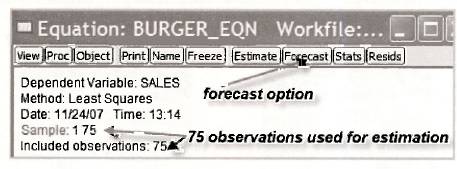
Now you are ready to compute the forecast. Go to your workfile and open the equation BURGER_EQN by double clicking on it. Then click on the forecast button in the toolbar. Before doing so, note that the number of observations used to estimate the equation is still 75. We are using the first 75 observations to estimate an equation which is then used to forecast sales for observation 76. Increasing the range of observations in a workfile does not change equations in the workfile that have already been estimated with fewer observations.

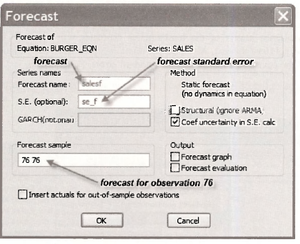
The following forecast dialog box appears. Let us consider the various items in this box.

Series names: The forecasts and their standard errors will appear in the workfile under the names SALESF and SE_F, respectively. The forecast standard error is computed using the formula on page 157 of the text. This formula includes what EViews calls Coef uncertainty in S.E. calculation. In this particular case, not including this uncertainty would mean the forecast standard error is the same as the standard deviation of the error term.

Forecast sample: We have chosen to forecast for just observation 76. We could have defined the forecast sample as 1 76, in which case EViews would produce both the in­sample forecasts as well as the out-of-sample forecast.

Method:       There are no dynamics in the equation because we do not have time series observations with lagged variables. These issues are considered in Chapter 9.

Output:         At this point we are not concerned with a Forecast graph, or a Forecast evaluation.

Insert actuals for out-of-sample observations: A tick in this box asks EViews to insert actual values for SALES, for the observations that lie outside your Forecast sample – in this case that would be observations 1 to 75. We did not choose this option.

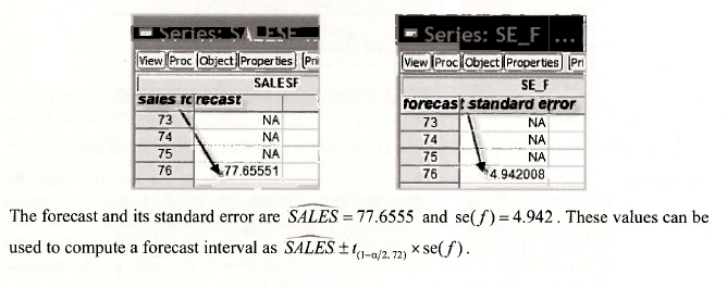
After clicking OK and closing the equation, you will be returned to the workfile where you will discover that SALESF and SE_F appear as two new series in the workfile. On opening these series by double clicking on them, you will further discover that the forecast and its standard error appear at observation 76, with the forecasts and standard errors at observations 1 to 75 being listed as NA, a consequence of the Forecast sample that we specified in the dialog box.

4. INTERVAL ESTIMATION

After obtaining least squares estimates of an equation we can proceed to use it for forecasting as we have done in the preceding section. In addition, we may be interested in obtaining interval estimates that reflect the precision of our estimates, or testing hypotheses about the unknown coefficients. The covariance matrix of the least squares estimates is a useful tool for these purposes, and one we will return to in Chapter 6. We begin by explaining how it can be viewed.

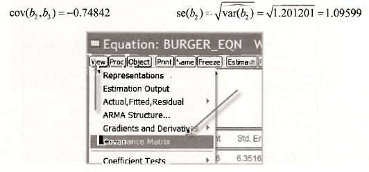
4.1. The least squares covariance matrix

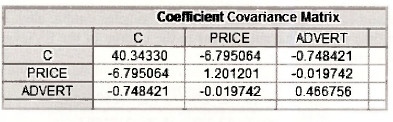
To examine the least squares covariance matrix go to the BURGER_EQN in your workfile and open it by double clicking. Select View/Covariance Matrix from the toolbar and drop-down menu. The covariance matrix of the least-squares estimates will appear. Check these values against those on p.l 16 of the text. Also note the relationship between the variances that appear on the diagonal of the covariance matrix and the standard errors. For example,

4.2. Computing interval estimates

A 100(1-a)% confidence interval for one of the unknown parameters, say β_k, is given by

Thus, to get EViews to compute a confidence interval, we need to locate values for b_k, se(b_k) and t_(1-a/2, _N-K) > ^ar|d then do the calculations. As we noted earlier in this chapter, the least squares estimates b_k will be stored in the object C in the workfile. Alternatively, they are stored in the array @coefs which was used for computing interval estimates in Chapter 3. That is, C = @coefs. If we are interested in one particular b_k, say b₂, then C(2) = @coefs(2) = – 7.907854. Similarly, the standard errors are stored in the array @stderrs, so that @stderrs(2) = 1.09599. Note that C, @coefs and @stderrs will contain values from the most recently estimated equation. If you are in doubt about their contents, quickly re-estimate the equation of interest. The remaining value that is required is /_{(1-a/2 N–K)}. It can be found using the EViews function @qtdistn(p,v) where p is equal to 1-a/2 and v is the number of degrees of freedom, in this case N – K = 15-3 = 12 . Putting all these ingredients together, upper and lower bounds for 95% interval estimates for P₂ and p₃ can be found from the following sequence of commands.

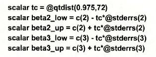
These commands are entered, one at a time, in the upper display of the EViews window. Each command is executed after you push the enter key. The answers are stored as scalars marked by S in the workfde.

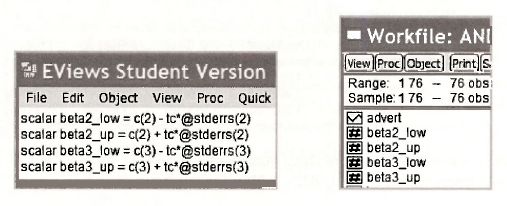
To view the upper and lower bounds of the interval estimates double click each of the scalars in the workfile. Each time the answer will appear in the bottom of the EViews window. Collecting these values one at a time, we obtain

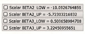
Apart from a small amount of rounding in the text values, you will discover that these interval estimates coincide with those on page 119 of the text.

5. HYPOTHESIS TESTING

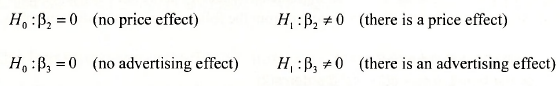
In this Chapter we are concerned with hypothesis tests on a single coefficient in the multiple regression model. More complex tests are deferred until Chapter 6. The most common single coefficient tests are two-tail tests of significance where, in the context of Andy’s Burger Bam, we are testing whether price effects sales and whether advertising expenditure effects sales.

5.1. Two-tail tests of significance

Two-tail tests of significance for the effect of price and the effect of advertising are considered on pages 121-2 of the text. The hypotheses for these tests are

Using EViews to calculate the /-values and p-values for these tests is trivial. They are automatically computed when you estimate the equation. To see where they are reported, we return to the least squares output for BURGER_EQN.

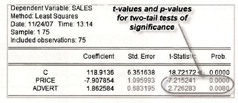
Do you know where these numbers come from? Consider the test for the effect of advertising. The t-value is given by t = 1.8626/0.6832 = 2.726. The p-value is given by

We can confirm the above result by asking EViews to compute the above probability using the command

scalar pee = 2*@ctdist(-2.726,72)

The function @ctdist(x, v) computes the distribution function value P[t_h) < x). The command can be entered in the top display of the EViews window. If you are unsure of how to do so, or how to read off the result, go back and check the earlier part of this chapter where we introduced a simple forecasting procedure, or the section where we computed interval estimates.

Knowing the p-value is sufficient information for rejecting or not rejecting H₀. In the case of advertising expenditure we reject H₀: β₃ = 0 at a 5% significance level because the p-value of 0080 is less than 0.05. Suppose, however, that we wanted to make a decision about H₀ by comparing the calculated value t = 2.726 to a 5% critical value. How do we find that critical value? We need values t_c and -t_c such that P(t₇₂ <t_c) = 0.975. Table 2 at the end of the book is not sufficiently detailed to provide this value. It can be obtained using the EViews command

scalar tc = @qtdist(0.975,72)

The answer is t_c = 1.993, a value that leads us to reject H₀: β = 0 because 2.726 > 1.993 .

The p-value for testing H₀: β₂ = 0 against H_x : P₂ * 0 is given as 0.0000 in the EViews regression output. As an exercise, use EViews to show that, using more decimal places, the value is 4.424 x 10^-10.

5.2. A one-tail test of significance

To collect evidence on whether or not the demand for burgers is price elastic, on pages 122-3 of the text we test H₀: β₂ > 0 against the alternative H₁: β₂ < 0 . In this case we are not particularly interested in the single point β₂ = 0, but, nevertheless, for testing H₀: β₂ > 0 we act as if the null hypothesis is H₀: β₂ = 0 . Thus, this test can be viewed as a one-tail test of significance. The p- value for this test is P[t₍₇₂₎ < —7.21524l) = 2.212x 10^-10. Because the calculated value t-value t = -7.215241 is negative, and the rejection region is in the left tail (as suggested by the direction of the alternative hypothesis H₁: β₂ < 0 ), we can compute the /(-value by taking half of the p- value given in the EViews regression output. However, since half of 0.0000 is 0.0000, this example is not a very interesting one. If we considered a one-tail test for advertising of the form H₀: P₃ < 0 against H_x : P₃ > 0, we could calculate its p-value as 0.0040, half of 0.0080.

If the calculated t- value is positive, and the rejection region is the left tail (or the calculated t- value is negative, and the rejection region is the right tail), the p-value will be greater than 0.5 and is not simply half of the EViews p-value. In such instances the p-value is given by p = 1 – p* /2 where p* is the EViews supplied p-value. Do you understand why? Check it out!

What is the 5% critical value for a one-tail test? For the case of β₂ where the critical value is a negative one in the left tail of the distribution, we can obtain it using the EViews command

scalar tc_1tail = @qtdist(0.05,72)

The value obtained is t_c =-1.666. Thus, making the test decision by reference to the critical value, we reject H₀: β₂ > 0 in favor of H₁ : β₂ < 0 because -7.215 < -1.666 .

5.3. Testing nonzero values

a. One-tail test

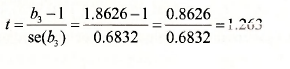
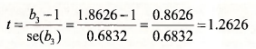
For advertising to be effective P₃ must be greater than 1. Thus we test H₀: β₃<1 against H₁: β₃>1. On page 123-4 of the text, we compute the key quantities for performing this test. They are the calculated t-value

and its corresponding p-value

You can compute these quantities using the following commands in the upper display of the EViews window.

scalar t3 = (c(3) -1 )/@stderrs(3)

scalar pee3 = 1 – @ctdist(t3,72)

b. Two-tail test

For two-tail tests there is an easier way to get the results from EViews. You can tell EViews the hypothesis that you want to test and it will do the rest. There is one temporary complication. EViews computes an F-value and a y -value but not a /-value. This complication will disappear once you have the extra background covered in Chapter 6. However, given that you are likely to be eagerly waiting to find out how EViews automatic testing commands work, we will give you some exposure now. If you are struggling with our explanations, please come back again after you have finished Chapter 6.

To illustrate we turn the recent hypothesis about the effect of advertising expenditure into a two-tail test, namely

H₀: β₃ = 1     against              H₁: β₃ # 1 

For testing this hypothesis, the calculated /-value is the same as before.

The ;p-value will be different, however. It is

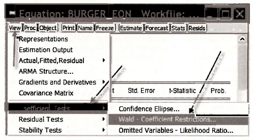
We have included more digits after the decimal so that we can match the accuracy of EViews. To get EViews to automatically compute these values, we proceed as follows. Open the equation object BURGER EQN and then select View/Coefficient Tests/Wald Coefficient Restrictions.

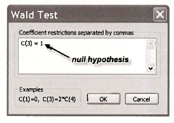
In the resulting dialog box type in the null hypothesis using the notation C(1) = β₁, C(2) = β_2, C(3) = β₃, and so on. For the null hypothesis H₀: β₃ = 1, we type c(3) = 1. Then click OK.

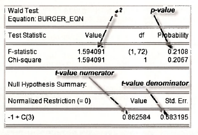
The following test results appear:

Note the following points:

1. The test is called a Wald test. The t-test and F-tests on the coefficients of regression equations belong to this class of tests. More details can be found on page 538 of the text.
2. In the last row of the output we can read off the numerator of the calculated t-value, namely b₃ -1 = 0.8626, as well as its standard error se(b₃ -1) = 0.6832 that appears in the denominator. Of course, se(b₃ -1) = se(b₃).
3. Instead of reporting the calculated value t = 1.2626, EYiews reports its square and calls it an F-value. That is, F = t² = 1.2626² =1.594. There is a theorem that says a t_{v) random variable squared is equal to an F_{(l v)} random variable. In words, the square of a / random variable with v degrees of freedom is equal to an F random variable with 1 degree of freedom in the numerator and v degrees of freedom in the denominator.

4. It is equally valid to perform a two-tail test with an F-distribution or a /-distribution. With one-tail tests squaring the /-value complicates matters. To avoid confusion, use the /- distribution.
5. The /?-value for the F-test is obtained from the right tail of its distribution. Specifically,

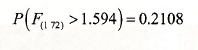
Because of the relationship between the t- and F-distributions, this p-value is identical to that obtained for the two-tail t-test and the same test conclusion is reached, namely, there insufficient evidence to reject H₀ at a 5% level of significance.

6. The EYiews output also reports a x² (chi-square) value. We will say more about this value in Chapter 6.

6. SAVING COMMANDS

Throughout this chapter we have entered a number of commands in the upper display of the EYiews window. It is a good idea to save these commands so that you have a record of them when you return to your work. To do so, highlight the commands and push Ctrl+C

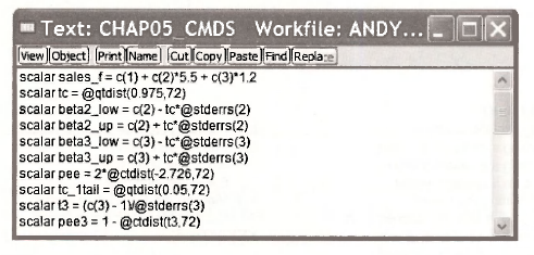
Then go Object/New Object and select the object Text. As a name for the object, enter CHAP05CMDS. After positioning the cusor within the Text dialog box push Ctrl+V. The following Text object will then be stored in your workfile

Source: Griffiths William E., Hill R. Carter, Lim Mark Andrew (2008), Using EViews for Principles of Econometrics, John Wiley & Sons; 3rd Edition.