Further Inference in the Multiple Regression Model by using EViews

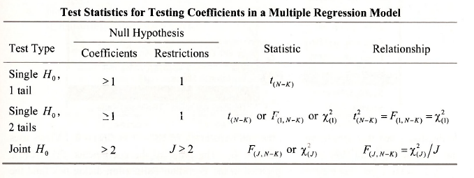
1. F AND CHI-SQUARE TESTS

In Chapter 5 we saw how to use EViews to test a null hypothesis about a single coefficient in a regression model. This test can be extended in two ways. We may want to test a single null hypothesis that involves two or more coefficients, or we might want to test a joint null hypothesis that specifies two or more restrictions on two or more coefficients. The choice of test statistic depends on whether the null hypothesis is single or joint and on whether the test is a one- tail test or a two-tail test. One-tail tests are only considered for single null hypotheses. In this case the relevant test statistic is t_(N__K). For two-tail tests of single hypotheses, we can use either the test statistic t_(N__K) or the statistic F_(1.N–K). The tests from each are equivalent because t²_(N__{K) =} F_(1.N–K) . An illustration was given in Section 5.5.3. Another test that can be used is a chi- square test that uses a chi-square statistic with one degree of freedom x²₍₁₎. The value of this statistic is identical to F_(1.N–K), but the test is different because a different distribution is used to compute the p-value. The A-test is an exact finite sample test suitable when the equation errors are normally distributed. The x² -test is an approximate large sample test that does not require the normality assumption. For joint null hypotheses the t-test is no longer suitable, nor do we consider one-tail tests. The alternative hypothesis H_l is that one or more of the restrictions in H₀ does not hold. We can use the F-test or the x² -test depending on whether or not we are invoking the normality assumption. The number of restrictions in H₀ gives the numerator degrees of freedom for the F-statistic and the degrees of freedom for the 7 -statistic. The two tests are different, but the value of one statistic can be calculated from the other using the relationship F(j,n-k) = x²_J/J.  All these different possibilities are summarized in the following table.

In the first part of this Chapter we use Andy’s Burger Barn example to demonstrate how these various testing scenarios can be handled within EViews. Our main focus will be on F- and x² – tests. You should check Chapter 5 for an introduction to the t-test.

The general formula for the F-value is

where SSE_R is the sum of squared errors from the model estimated assuming the restrictions in H₀ hold and SSE_U is the sum of squared errors from the unrestricted model. The corresponding X² -value is given by x² = J x F . We can use EViews to compute F and x² and their p-values automatically or we can use EViews to compute the restricted and unrestricted models, locate SSE_r and SSE_U on the output, and then calculate F and x².

1.1. Testing significance: a coefficient

Our first example is to test H₀: β₂ = 0 against the alternative H₁: β₂ # 0 in the model

In other words, should PRICE be included in the equation? We used a t-test to perform this test in Section 5.5.1; we discovered we could read the result directly from the regression output. Let us see how we can do it using F- and x² -tests.

a. Using E Views test option

Return to the workfile andy.wfl and open the equation object BURGER_EQN. Select View/Coefficient Tests/Wald Coefficient Restrictions

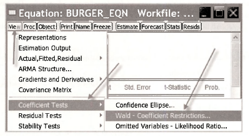
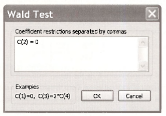
In the dialog box that appears we type the null hypothesis H₀: β₂ = 0 as C(2) = 0. EViews uses the notation C(k) to denote the coefficient B_k. The order of the coefficients C(1), C(2), C(3),… is the order that they were specified in the Equation Estimation dialog box (and the order in which they appear in the regression output).

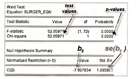
Clicking OK yields the output that appears below. You should note the following:

1. The test is called a Wald test. The t-test and F-tests on the coefficients of regression equations belong to this class of tests. More details can be found on page 538 of the text.
2. The Normalized Restriction (=0) in the bottom part of the table refers to the null hypothesis rearranged so that the right-hand side of the restriction in H₀ is zero. In this particular example no rearrangement is necessary because the right-hand side of H₀: β₂ = 0 is already zero.
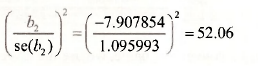
3. Value and Std.Err. of the Normalized Restriction refer to the estimated value of the left-hand side of the rearranged H₀ and its standard error. In this case these values are b₂ = -7.907854 and se(b₂) = 1.095993.

4. The calculated F- and x²-values are approximately F = x² =52.06. They are identical because there is only one restriction in H₀ (J = 1). And they are equal to the square of the /-value for testing this hypothesis. That is,
5. The degrees of freedom (df) are (1,72) for the F-test and 1 for the x² -test.
6. The reported p-values for each of the tests are both 0.0000. Thus, we reject H₀: β₂ = 0 at all reasonable significance levels.

b Using the formula for F

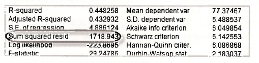
To perform the test using the formula for F we need the quantities SSE_U and SSE_R. We can read SSE_U =1718.943 from the regression output:

After estimation EViews stores this quantity as @ssr, short for “sum of squared residuals”. Since the text uses SSR for “regression sum of squares”, this notation can be confusing. Be careful! We can call it something more familiar by using the EViews command

scalar sse_u = @ssr

To find SSE_r we estimate the model under the assumption that H₀: β₂= 0 is true. This model is

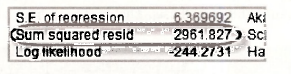
Using EViews to estimate this model we find SSE_R = 2961.827 which can be read directly from the regression output.

To save this quantity using a convenient name, we use the EViews command

scalar sse_r = @ssr

Then, the required F-value is given by

scalar f_val = (sse_r – sse_u)/(sse_u/(75-3))

A check of this calculated value shows it is the same as that obtained using EViews’ test option.

To finalize the test we need either the p-value or the critical value. These values can be obtained using EViews commands for the F distribution function and the F quantile function. For the p- value we have

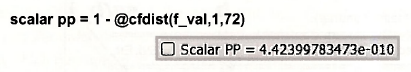
For the critical value we have

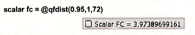
Again, we are led to reject H₀. Note that that the p-value is the same as that on page 121 of the text where a t-test was performed. Also the critical value is equal to the square of the t critical value: F = 3.9739 = t²_c = 1.99346²

What about the x² -test? The x²-value is the same as the F, that is, x² = 52.06 . Its p and critical values can be found using EViews commands for the x² distribution function and the x² quantile function.

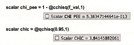
Note that the p-values from the F- and x²-tests are different, although the test conclusion is clearly the same.

1.2. Testing significance: the model

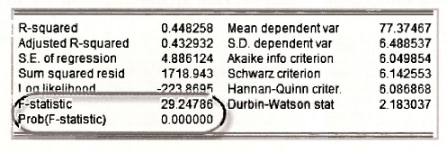
The F-test for testing the significance of a model is given special prominence in the regression output. In the context of Andy’s Burger Bam the hypotheses for this test are

The null hypothesis is a joint one because there are 2 restrictions P₂ = 0 and P₃ = 0. The restricted model that assumes H₀ is true is

This model has no explanatory variables. Testing the significance of a model is equivalent to testing whether any of the explanatory variables influences the dependent variable. The sum of squared errors for the unrestricted model is the same as before, SSEy =1718.943. The sum of squared errors for the restricted model is equal to the sum of squared deviations of SALES around its mean, also known as the total sum of squares (TSS). This result holds because the restricted least squares estimator for P, is the sample mean for SALES. Note that TSS for a series y is given by

The EViews functions for y and ^yf are @mean(.) and @sumsq(.), respectively. Using this information, a sequence of EViews commands that computes the required F-value and its /j-value are

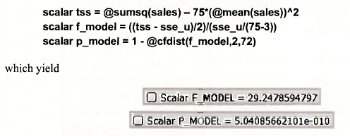
In practice there is no need to go through this sequence of calculations. The F- and p-values are automatically reported on the BURGER_EQN regression output.

2. TESTING IN AN EXTENDED MODEL

2.1. Estimating the model

On page 140 of the text Andy’s Burger Barn model is extended to also include the square of advertising expenditure as one of the explanatory variables. The new model is

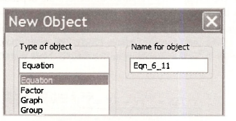
To estimate this model we begin by selecting Object/New Object and choose Equation from the menu of objects. We have named the equation EQN_6_11 in line with equation number on page 141 of the text.

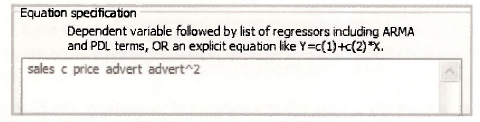
The names of the series are entered in the Equation specification dialog box, with the dependent variable SALES., appearing first, followed by the constant C, then the explanatory variables PRICE, ADVERT and ADVERT². Notice that it is legitimate to write simply advertˆ2 for ADVERT². An alternative way is to define a new series, say

series advert2 = advertˆ2

and include advert2 as one of the explanatory variables.

The Estimation settings remain as before with Least Squares being the Method and 1 75 for the Sample.

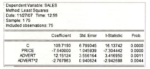
The following results appear. Check them against those on page 141 of the text.

2.2. Testing: a joint H₀, 2 coefficients

Since advertising appears twice in the equation, as ADVERT and as ADVERT², to test whether advertising has an effect on sales we need to test H₀: β₃ = 0 and β₄ = 0 against the alternative H₁: β₃ # 0 and β₄ # 0, as described on page 142 of the text. The null hypothesis is called a joint null hypothesis because it contains two restrictions. To get EViews to perform the test go to the EViews workfile and open the equation object EQN_6_11. Then, select View/Coefflcient Tests/Wald Coefficient Restrictions

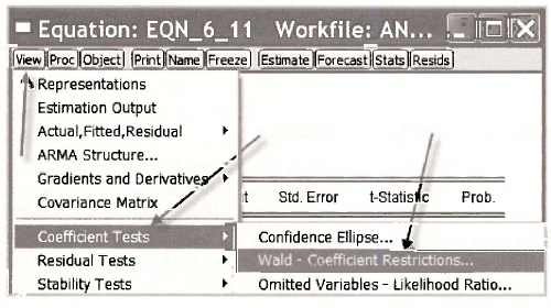
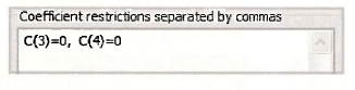
In the resulting Wald Test dialog box enter the two restrictions C(3) = 0, C(4) = 0 and click OK.

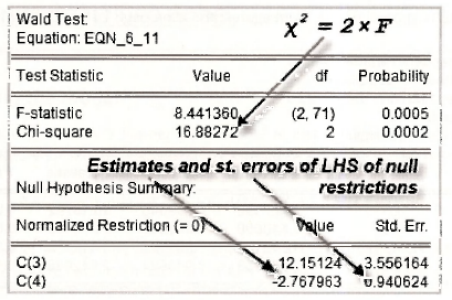
The above output contains the following information.

1. The Normalized Restriction (=0) in the bottom part of the table refers to the two restrictions in the null hypothesis rearranged so that their right-hand sides are zero. In this particular example no rearrangement is necessary because the right-hand sides are already zero and the left-hand sides are simply β₃ and β₄.
2. Value and Std. Err. of the Normalized Restriction refer to the estimated values of the left-hand sides of the rearranged restrictions and their standard errors. The values are b₃ = 12.151 and b₄ = -2.7680, with standard errors se(b₃) = 3.556 and se(b₄) = 0.9406 .
3. The calculated F- and yj-values fortesting H₀ are F = 8.441 and x² =16.883. Because there are 2 restrictions, x² = 2 x F .
4. The degrees of freedom (df) are (2,71) for the F-test and 2 for the x² -test.
5. The reported p-values for F- and x² -tests are 0.0005 and 0.0002, respectively. Thus, we reject H₀: β₃ = 0 and β₄ = 0 at all conventional significance levels.

2.3. Testing: a single H₀, 2 coefficients

On page 143-4 of the text both a t-test and an F-test are used to test whether ADVERT = 1.9 is the optimal level of advertising. We will show how EViews automatic commands can be used to perform F- and x² -tests and how, along the way, information for the f-test is produced. Performing the f-test requires one to compute the standard error for a linear function of two coefficients. We illustrate how this value can be read from the EViews test output as well as how to calculate it from the EViews coefficient covariance matrix.

The null and alternative hypotheses are

In the Wald Test dialog box the restriction in H₀ is entered as

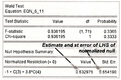
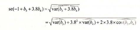
To write H₀: β₃ + 3.8β₄ = 1 as a Normalized Restriction (=0), EViews moves 1 from the right- hand side to the left-hand side, giving the normalization H₀ :-1 + β₃ + 3.8β₄ = 0. Value is an estimate of the left-hand side, namely, -1 + b₃ +3.8b₄ =0.632976. Std. Err. refers to se(-1 + b₃ +3.8b₄) = 0.65419. It is calculated by EViews using the formula

The calculated F- and x²-values for testing H₀ are F = x² =0.9362. They are both the same because there is only one restriction. The degrees of freedom (df) are (1,71) for the T’-test and 1 for the x²-test. The reported p-values for F- and x² -tests are 0.3363 and 0.3333, respectively. Thus, we do not reject H₀ at a 5% significance level. The p-values can be confirmed with the commands

scalar p_f_o = 1 – @cfdist(0.936195,1,71)

scalar p_chi_o = 1 – @cchisq(0.936195, 1)

Notice that the EViews output also gives enough information to perform a t-test. The required test value is given by

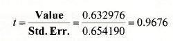
Because t² = 0.9676² = 0.936 = F, for a two-tail test there is no need to consider both t-and F- tests. Both give the same result. Flowever, the information for the t-test is useful for one-tail tests as described on page 145 of the text.

a. Standard error for a linear function of coefficients

It is instructive to see how to compute the standard error se(b₃ + 3.8b₄) = 0.65419 from the least squares covariance matrix. After estimating equation (6.11) and saving it as the equation object EQN611, the covariance matrix for the least squares estimates is stored as a symmetric matrix called eqn_6_11.@cov. A symmetric matrix is a square array of numbers where the values above the diagonal are equal to the corresponding ones below the diagonal. If the columns are made rows and the rows are made columns, we get the same array. A covariance matrix is always symmetric because cov(b_k,b₍) – co\(b_nb_k) for any two coefficients b_t and b_k. EViews refers to symmetric matrix objects as sym. Thus, to list the least squares covariance matrix in our workfile with the name covb, we use the command

sym covb = eqn_6_11.@cov

The command to compute and save it in the workfile with name vee is

scalar vee = covb(3,3) + 3.8^ˆ2*covb(4,4) + 2*3.8*covb(3,4)

and the standard error, called se_o, is

scalar se_o = @sqrt(vee)

Following these steps will give the value se(b₃ + 3.8b₄) = 0.65419.

b. Using restricted and unrestricted SSE

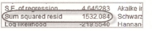
On page 144 of the text, the F-value for testing the optimality of advertising expenditure is computed using SSE_V and SSE_R. As we have seen, it is more easily computed using EViews automatic test option. Nevertheless, we will show you how the values for SSE_V and SSE_R can be obtained. The value SSE_V =1532.084 is located from the output for EQN_6_11.

The value SSE_R = 1552.286 is obtained by estimating the model

(SAFES – ADVERT) = β₁+ β₂PRICE + β(AADVERT² -3.8x ADVERT) + e

To estimate this model we use the following Equation specification.

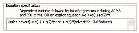
Take another look at this box. The way the equation is entered is very different from what we have seen so far. Before when we specified the equation we simply listed the dependent variable followed by the constant and the explanatory variables. Here we have written out the equation in full using C( 1), C(2) and C(4) to denote P,, P₂ and P₄. This is another way that an equation can be specified in the Equation specification dialog box. It is convenient in this instance because of the way we have rearranged the equation. It produces the following output.

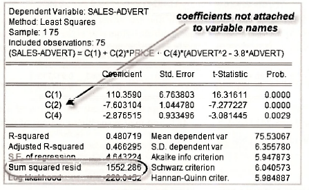
For testing purposes, the value SSE_R =1552.286 is of interest. However, notice also that the coefficients are listed as C( 1), C(2) and C(4) instead of by the names of the variables to which they are attached. In this case there are not unambiguous variable names that can be attached to the coefficients.

2.4. Testing: a joint H₀, 4 coefficients

The final example of a test using the extended hamburger model is on page 145 of the text. Here we are concerned with testing the joint null hypothesis

They are entered in the Wald Test dialog box in the following way.

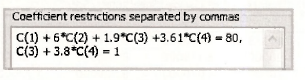
In the output that follows EViews has written these restrictions in the normalized formats -1 + β₃ + 3.8β₄ = 0 and -80 + β₁+6β₂+1.9β₃+3.61β₄ =0 . Note that the EViews output has abbreviated the latter of these two restrictions. Their estimated values and the corresponding standard errors found in the bottom part of the output are

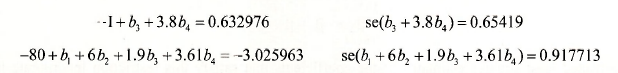
As expected, the values for the restriction considered in the previous section have not changed.

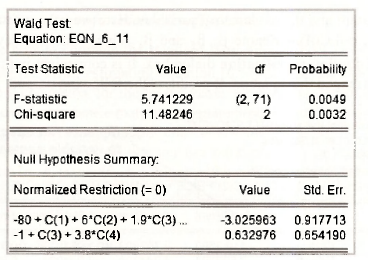
The test values F = 5.7413 and x² = 11.482, and their respective ^-values of 0.0049 and 0.0032, lead to rejection of H₀ at a 5% significance level.

3. INCLUDING NONSAMPLE INFORMATION

The model used on page 146 of the text to illustrate the inclusion of nonsample information is the demand for beer equation

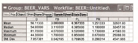
where Q is quantity demanded, PB is the price of beer, PL is the price of liquor, PR is the price of remaining goods and services and / is income. The data are stored in the file beer.wfl. Before proceeding with estimation, we check the summary statistics in Table 6.1. Open the file, create a group of variables as described in Chapter 5, and select View/Descriptive Stats/Common Sample.

The nonsample information, that economic agents do not suffer from “money illusion”, can be expressed as

Restricted least squares estimates of the coefficients that satisfy this restriction incorporate the nonsample information.

Several examples of restricted least squares estimation were given in the previous section. Each time we estimate a model assuming a null hypothesis is true we are finding restricted least squares estimates. In Section 6.2.4 we used the restrictions to rearrange the equation, and estimated the rearranged equation. The same thing can be done in this case. Indeed, the rearranged equation appears as (6.18) and (6.19) in the text. As an exercise, we recommend that you use EViews to estimate (6.18) and confirm the results presented in (6.19).

To broaden your EViews experience, we will do it another way. Instead of estimating the rearranged equation, it is possible to simply substitute the restriction into the equation. EViews is smart enough to estimate it without you worrying about how to rearrange it. Substituting the restriction in to the equation yields

This equation can be written into the Equation specification dialog box as follows

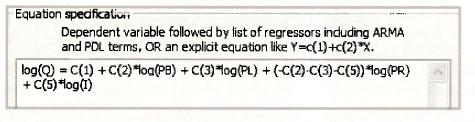
Notice that the equation has been written in full. It is not just a list of variables. The resulting output follows. The values are consistent with those in equation (6.19) of the text.

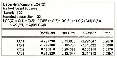
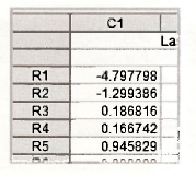
The value for b*_A can be retrieved using the command

c(4) = – c(2) – c(3) – c(5)

Checking the C object yields the complete set of estimates

4. THE RESET TEST

In Section 6.6 of the text, an example that relates family income to husband’s education, wife’s education and number of children is used to illustrate the effects of omitted and irrelevant variables. Various equations are estimated, summary statistics are given, including the correlation matrix of the variables, and the RESET test is introduced as a device for discriminating between models. We will not dwell on how to estimate the various equations. To do so is straightforward given the material you have covered so far in Chapters 5 and 6. Finding the correlation matrix for the variables is new, and important. It helps explain the effect of omitted and irrelevant variables and it is useful for detecting collinearity, a topic considered in Section 6.7. However, at this point it is convenient to defer reproducing Table 6.2 on page 149 until the next section where we also consider the correlation matrix for the variables in a gasoline consumption example. In this section our current focus is on how to get EViews to compute test statistic values for the RESET test. The model we consider is

where FAMINC is family income, HEDU is husband’s education, WEDU is wife’s education and KL6 is the number of children in the household who are less than 6 years old. To perform the RESET test we estimate this equation, obtain the predictions FAMINC, then estimate one or both of the following models

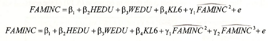
RESET tests are F-tests for H₀: y, = 0 or H₀: y_l = 0 and y₂ = 0 . Rejection of either H.₀ implies the specification of the equation can be improved. The tests can be performed in the same way as the F-tests described earlier in this Chapter, but in this case EViews has special capabilities which require less effort. We will consider the special capabilities (the short way) as well as a long way that reinforces the fundamentals of the test.

4.1. The short way

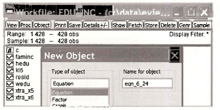
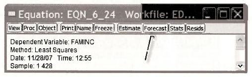
Open the workfile edu_inc.wfl. Create an equation object called EQN_6_24.

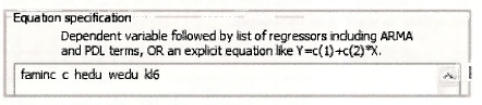
Enter the variables in the Equation specification dialog box.

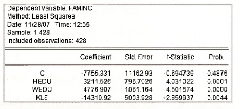
The estimated equation, in line with (6.24) on page 150 of the text, is

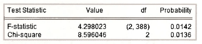
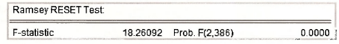
With this equation open, go to View/Stability Tests/Ramsey RESET Test.

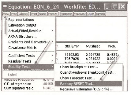
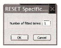
A dialog box will ask you for the number of fitted terms. Inserting 1 leads to the model with FAMINC². Inserting 2 gives you the model with both FAM1NC² and FAM1NC³ included.

Clicking OK gives detailed output from estimating the specified test equation. Because most of this output should be meaningful to you by now, we will focus just on the F- and /(-values for the tests. These values appear at the top of the output.

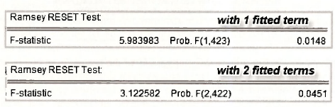
In both cases the null hypothesis of no specification error is rejected at a 5% level of significance. Improvements to the model should be possible.

4.2. The long way

After estimating the basic equation go to Forecast.

Give the forecasts a name such as FAMINC_HAT. The Forecast sample is the same as the sample used for estimation, 1 428.

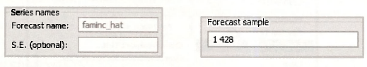
The series FAMINC_HAT will appear in your workfile. Estimate the equation with one fitted term.

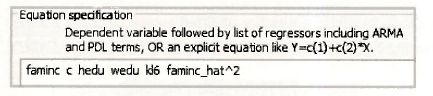
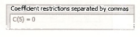
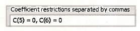
In the output that follows, go to View/Coefficient Tests/Wald – Coefficient Restrictions. Insert ^c(5) = 0 as the hypothesis to test. The test result will agree with that obtained the short way.

Now estimate the equation with two fitted terms.

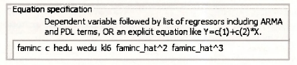
In the output that follows, go to View/Coefficient Tests/Wald – Coefficient Restrictions. Insert c(5) = 0, c(6) = 0 as the hypothesis to test. The test result will agree with that obtained the short way.

5. VIEWING THE CORRELATION MATRIX

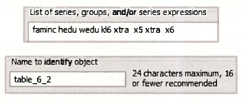
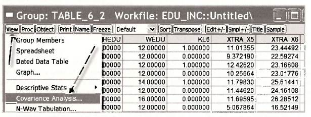
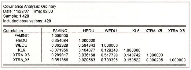
The matrix of correlations between explanatory variables is an important tool for assessing the sensitivity of results to inclusion or exclusion of variables and the likely causes of imprecise estimates. To obtain the correlation matrix for the variables in the file edu inc.w/1, we begin by creating a group object containing those variables. Suppose that group has been created and, in line with page 149 of the text, we call it TABLE 6 2.

To view the correlation matrix of the variables in the group, go to View/Covariance Analysis.

In the Covariance Analysis dialog box that follows, you will find a large number of options. At present we are only interested in correlation presented as a single table. Our method is ordinary and we have a balanced sample.

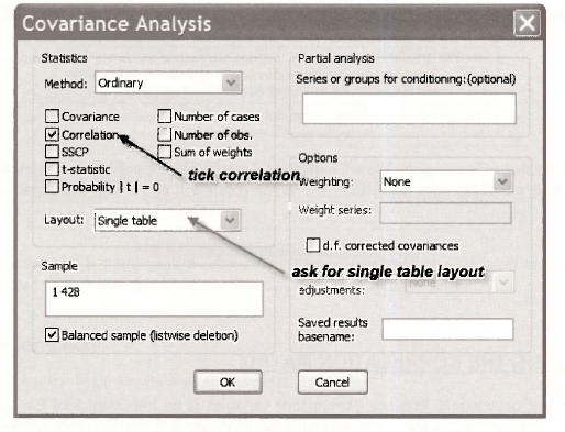
Clicking OK produces the following table. Check it against Table 6.2 on page 149 of the text.

5.1. Collinearity: an exercise

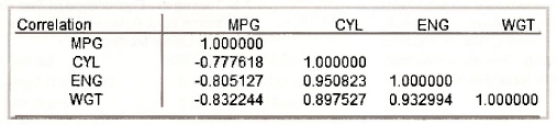
The final example in Chapter 6 is described on pages 154-5 of the text. It involves a model for gasoline consumption, used to illustrate the effects of collinearity. The data are stored in the workfile cars.wfl. Because the information provided in the text can all be obtained using EViews commands that we have covered earlier, this example is a good candidate for an exercise. Check your EViews skills by answering the following questions.

1. Estimate the two equations on page 155 of the text. Check your estimates, standard errors and p-values against those that are reported.
2. Consider the model

Show that the test results for testing H₀: β₂ = 0 and β₃ = 0 are

3. Show that the RESET test result (with two-fitted terms) for this model is

What do you conclude?

4. Show that the correlation matrix for the variables is

 

Source: Griffiths William E., Hill R. Carter, Lim Mark Andrew (2008), Using EViews for Principles of Econometrics, John Wiley & Sons; 3rd Edition.