1. PREDICTION IN THE FOOD EXPENDITURE MODEL
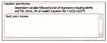
In this chapter we continue to work with the simple linear regression model and our model of weekly food expenditure. To begin, open the food expenditure workfile food.wfl. On the EViews menu choose File/Open and then open the file. So that the original file is not altered save this under a new name. Select File/Save As then name the file food_chap04.wfl. Estimate the simple regression
![]()
The estimation can be carried out by entering into the command line
Is food_exp c income
Alternatively, on the EViews menu select Quick/Estimate Equation, then fill in the dialog box with the equation specification and click OK.
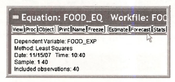
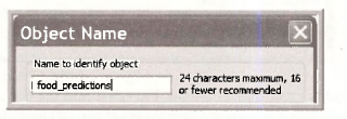
Name the resulting regression results FOOD_EQ by selecting the Name button and filling in the Object name.
1. A simple prediction procedure
In Chapter 2.8 of this manual we illustrated a simple procedure for obtaining the predicted value of food expenditure for a household with income of $2,000 per week. We also showed that EViews can be used to generate forecasts automatically, both the for sample values and for new INCOME observations that we append to the workfile by increasing its range. If you need to review those steps do so now.
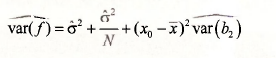
What we can add now that we did not have before is the standard error of the forecasted value. The estimated variance of the forecast error is
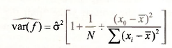
A convenient form for calculation in the simple regression model is
Open the food equation FOOD_EQ. Click on View/Representations. Select the text of the equation listed under Substituted Coefficients. We can choose Edit/Copy from the EViews menubar, or we can simply use the keyboard shortcut Ctrl+C to copy the equation representation to the clipboard. Finally, we can paste the equation into the command line.
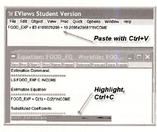
To obtain the predicted food expenditure for a household with weekly income of $2000, edit the command line to read
scalar food_exp_hat = 83.4160020208 + 10.2096429681*20
Press Enter. The resulting scalar value is
![]()
which is correct to more decimals than the value 287.61.
The prediction interval requires the critical value from the r{38) distribution. For a 95% prediction interval the required critical value is tc is the 97.5-percentile, which is obtained as
scalar tc = @qtdist(.975,38)
The prediction interval is obtained by entering the following commands (do not type the comments in italic font).
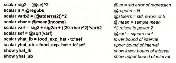
The resulting prediction interval values are:
![]()
These results are correct, but obtaining a prediction interval this way each time would be tedious. Now we use the power of EViews.
2. Prediction using EViews
The above procedure for computing a prediction interval works for the simple regression model. EViews makes computing standard errors of forecasts simple. In Section 2.8.2 of this manual we extended the range of the workfile and entered 3 new observations for INCOME = 20, 25 and 30. Follow those same steps again to insert the same three observation values. The steps are:
- Double click on Range in the main workfile window.
- Change the number of observations to 43 and click
- Double click on INCOME in the main workfile to open the series.
- Click Edit+/- to open edit mode.
- Enter 20, 25 and 30 in cells 41-43.
- Click Edit+/- to close edit mode.
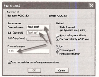
In the FOOD_EQ window click on Forecast
In the dialog box that opens enter names for the Forecast and the S.E., which is for the standard error of the forecast. Make sure the forecast sample is set to 1 -43 and click OK.
The resulting window shows the predicted values and a 95% prediction interval for the observations in their given order. For cross sectional observations this is not so useful. We will come back to it later.
Enter the following commands into the command line, or use the Genr button to open a dialog box in which the new series can be defined.
series food_exp_ub = food_expf + tc*food_sef
series food_exp_lb = food_expf – tc*food_sef
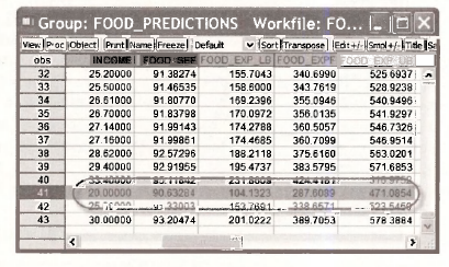
Create a group by clicking on INCOME., FOOD SEF, FOOD EXP LB, FOOD EXPF, FOOD EXP UB. To do this, click each one while holding down Ctrl. Right click in the shaded area and select Open/ as Group.
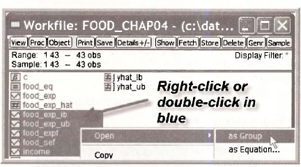
Click on Name and call this group FOOD_PREDICTIONS.
Scroll to the bottom to see the standard error of the forecast and prediction intervals for the specified values of income. Note that the value for = 20 are as we constructed manually.
2. MEASURING GOODNESS-OF-FIT
2.1. Calculating R2
The usual R1 = 1 – SSE/SST is reported in the EViews regression output. In the FOOD EQ window it is reported just below the regression coefficients
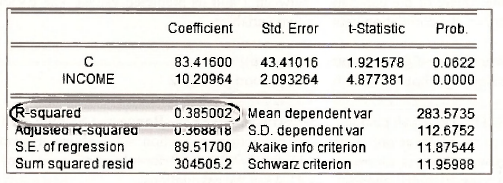
The elements required to compute it in this window are shown as well. The sum of squared least squares residuals (SSE) is given by
Sum squared resid 304505.2
The total sum of squares (SST) can be obtained from
S.D. dependent var 112.6752
Recall that the sample standard deviation of the y values (S.D. dependent var) is
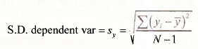
Thus if we square this value, and multiply by N- 1 we will have it. That is
![]()
You can do this by hand, or recall that after a regression model is estimated many useful items are saved by EViews, including
@sddep standard deviation of the dependent variable
@ssr sum of squared residuals
Then, to calculate R2 use the commands
scalar sst = (N-1)*(@sddep)ˆ2
scalar r2 = 1-@ssr/sst
The value ‘N had already been calculated as
scalar n = @regobs
2.2. Correlation analysis
In the simple regression model we can compute R2 as the square of the correlation between X and Y or the square of the correlation between Y and its predicted values. The EViews function @cor computes the correlation between two variables.
scalar r2_xy=(@cor(income,food_exp))ˆ2
scalar r2_yyhat = (@cor(food_exp, food_expf))ˆ2
3. MODELING ISSUES
3.1. The effects of scaling the data
Changing the scale of variables in EViews is very simple. Generate new variables that have been redefined to suit you. To illustrate, suppose we measure INCOME in $ rather than in 100$ increments. That is, we prefer the variable DOLLAR INC = 100 * INCOME. Create this new variable by clicking the Genr button, then enter
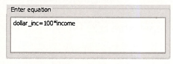
and click OK. Alternatively, on the command line, enter
series dollar_inc=100*income
Estimate the food expenditure model using this new variable. Click Quick/Estimate Equation and enter
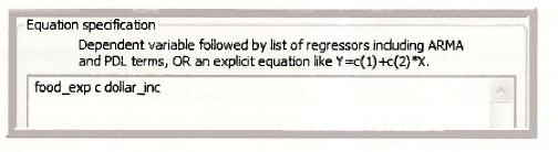
Click OK Alternatively, on the command line enter
Is food_exp c dollar inc
The result is
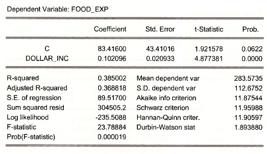
The coefficient on income has changed, as has its standard error. Everything else in this regression is the same as earlier estimations of the food expenditure equation.
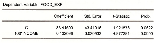
A useful feature of EViews is that the regression commands allow variables to be transformed directly. That is we could obtain the same results by entering
Is food_exp c (100*income)
The regression coefficients are now
3.2. The log-linear model
To use logarithmic transformations recall that the EViews function log represents the “natural logarithm” that we denote in POE as “In”. To estimate the log-linear version of the food expenditure model first generate the log of the dependent variable,
series lfood_exp = log(food_exp)
Recall that transforming the dependent variable in this way fundamentally changes how the results are interpreted. In the equation ln(y) = P, +fi2x + e, a 1-unit increase in “x” leads to a 100P2% increase in the expected value ofy.
Now, use this dependent variable in the regression model,
Is lfood_exp c income
The results are
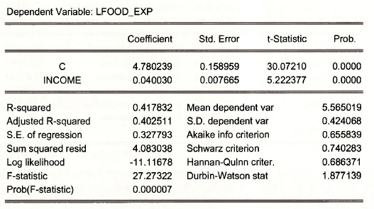
We would interpret this by saying that an increase in income of $100 (1-unit) leads to about a 4% increase in food expenditure. Because we have transformed the dependent variable in this way, the Rz changes and is not comparable to earlier estimations. More on this later.
Instead of creating lfood_exp = log(food exp) we could have specified the transformation directly in the regression statement, as
Is log(food_exp) c income
3.3. The linear-log model
The linear-log model transforms the x variable, but not the y variable: v = P, + P2 \n(x) + e . In this model a 1% increase in x leads to a P2/100 unit change in y. In the food expenditure model the commands are
series lincome = log(income)
Is food_exp c lincome
The resulting regression output is:
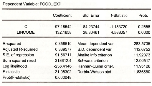
We would interpret the results by saying that a 1% increase in income leads to about a $1.32 increase in weekly food expenditure.
The linear-log model can be estimated directly as
Is food_exp c log(income)
3.4. The log-log model
In the log-log model ln(y) = pj+p2 ln(x) + e the parameter P2 is an elasticity. For the food expenditure model, using the log-variables we have already created, the regression command is
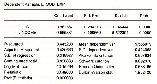
Is lfood_exp c lincome
The result is shown on the next page. A 1% increase in income leads to about a ‘/i% increase in food expenditure. Alternatively use the regression command
Is log(food_exp) c log(income)
3.5. Are the regression errors normally distributed?
Each time a regression is estimated a certain number of regression diagnostics should be carried out. It is through the residuals of the fitted model that we may detect problems in a model’s specification. One aspect of the error that we can examine is whether the errors appear normally distributed. EViews reports diagnostics for the residuals each time a model is estimated. For example, in the FOOD EQ window, select View/Residual Tests/Histogram-Normality Test
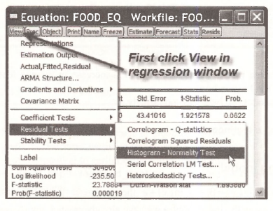
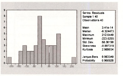
A Histogram is produced along with other summary measures. The Mean of the residuals is always zero for a regression that includes an intercept term. In the histogram we are looking for a general “Bell-shape”, and a value of the Jarque-Bera test statistic with a large /3-value. This test is valid in large samples, so what it tells us in a sample of size A = 40 is questionable. The test statistic has a yf„, distribution under the null hypothesis that the Skewness is zero and Kurtosis
is three, which are the measures for a normal distribution. The critical value for the chi-square distribution is obtained by typing into the command line
=@qchisq(.95,2)
which produces the scalar value
![]()
Save your workfile and close it, as we are moving to another example.
3.6. Another example
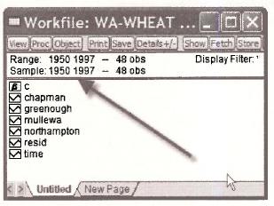
Open the workfile wa-wheat.wfl by selecting on the EViews menu File/Open/EViews Workfile. Locate wa-wheatwfl and click OK. It contains 48 annual observations on the variables NORTHAMPTON, CHAPMAN, MULLEWA, GREENOUGH. and TIME. The first 4 variables are average annual wheat yields in shires of Western Australia. See the definition file wa-wheat.def These are annual data from 1950 to 1997
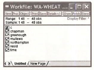
Before working with the data, double-click on Range. This will reveal the Workfile structure. When this file was created the annual nature of the data and time span were not used.
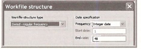
In the Date specification choose an Annual frequency with Start date 1950 and End date 1997, then OK.
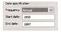
This will not have any impact on the actual results we obtain, but it is good to take advantage of the time series features of EViews. The resulting workfile is now
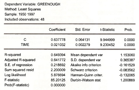
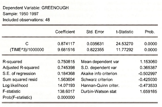
Save this workfile with a new name. Select File/Save As to open a dialog box. We will call it wheat chap04. Estimate the linear regression of YIELD in GREENOUGH shire on TIME by entering
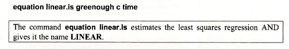
Alternatively use the usual Quick/Estimate Equation dialog box, and then name the result.
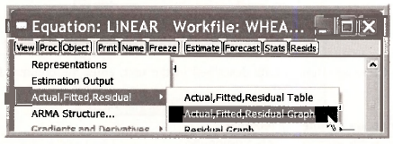
In the regression results window, click on View/Actual,Fitted,Residual/ Actual,Fitted,Residual Graph to construct Figure 4.8 in POE.
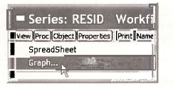
The bar graph in Figure 4.9 of POE is obtained by opening (double-click) the series RESID in the workfile window. Recall that EViews always saves the most recent regression residuals as RESID. In the spreadsheet view click View/Graph
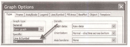
In the Graph Options window choose Bar as the Specific type of graph.
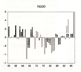
The result is shown below. The advantage of specifying that the data series is Annual with specified dates is that EViews then labels the horizontal axis with the years.
To generate the cubic equation results described in the text, enter the commands (or use drop down boxes)
genrtimecube = (timeˆ3)/1000000
equation cubic.ls greenough c timecube
Or use the single command
equation cubic.ls greenough c (timeˆ3)/1000000
This workfile (wheat_chap04.wfl) can now be saved and closed.
4. THE LOG-LINEAR MODEL
To illustrate the log-linear model we will use the workfile cps smalLwfl, with data definitions in cps smalLdef. This data file consists of 1000 observations.
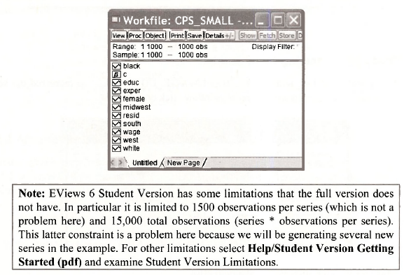
To prevent a problem delete all the series except WAGE and EDUC. To do this, click on each series while holding down Ctrl. Right-click in the blue area and select Delete. Save the workfile with a new name, such as wage_chap04.wfl, because we will use the data to estimate a wage equation.
Create a new series that is In (WAGE) and estimate the log-linear equation.
series Iwage = log(wage)
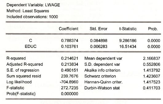
equation lwage_eq.ls Iwage c educ
Note that we have given the Name LWAGE_EQ to this equation.
4.1. Prediction in the log-linear model
First we illustrate prediction with the equation LWAGE_EQ in which we regressed the series LWAGE on EDUC. In the estimated equation window click on Forecast.
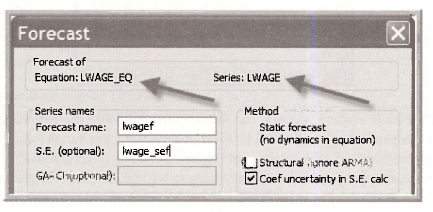
Select names for both the forecast and standard error.
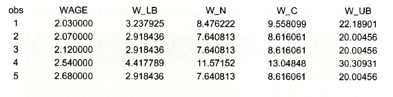
To create a prediction interval for the predicted value of WAGE, we first create a 95% interval for LWAGEF as the forecast plus and minus the /-critical value times the standard error of the forecast. Then to convert if from logs to a numerical scale we take the antilog using the exponential function. The following commands create the /-value and the upper and lower bounds of predicted wage.
scalar tc = @qtdist(.975,998)
series w_ub = exp(lwagef + tc*lwage_sef)
series w_lb = exp(lwagef – tc*lwage_sef)
In repeated samples this prediction interval procedure will work 95% of the time. If however we seek a single predicted value, rather than an interval, it is possible that an alternative predictor, based on the properties of the log-normal distribution may be better. The natural predictor is the anti-log of the predicted log(wage)
series w_n = exp(lwagef)
In large samples a more precise predictor is obtained by correcting for log-normality, to do so we multiply the natural predictor by exp(σ2/2). The value of the estimated σ is saved after a regression as @se. Thus the corrected predictor is
scalar sig2 = (@se)ˆ2
series w_c = exp(lwagef)*exp(sig2/2)
A few values of the actual wage, the prediction interval, and the natural and corrected predictors are shown below. Note that the corrected predictor is always going to be larger than the natural predictor because the correction factor is always larger than one.
4.2. Alternative commands in the log-linear model
EViews allows transformations of variables to be included in the statement of the regression model, so instead of creating a new variable LWAGE as we did in Section 4.4.1, we can enter the statement
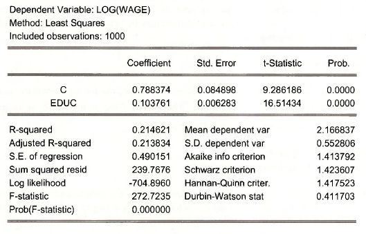
equation wage_eq.ls log(wage) c educ
Or, in the Quick/Estimate Equation dialog box enter the Equation specification
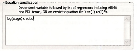
then name the equation WAGE_EQ. Either way, the results are as shown below.
In the WAGE EQ window select Forecast. Choose the LOG(WAGE) radio button
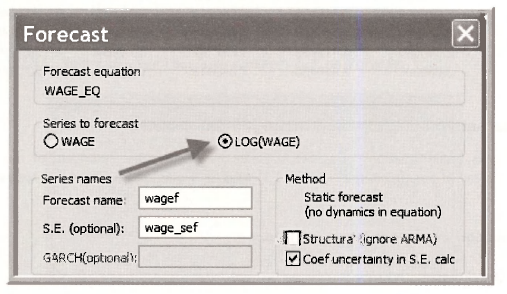 The series WAGEF and WAGE SEF will be equal to series LWAGEF and LWAGE SEF, respectively. Then proceed with prediction interval calculations as in Section 4.4.1
4.3. Generalized R2
A generalized goodness of fit measure is the squared correlation between the actual value of the dependent variable and its best predictor. Using the EViews function @cor, we obtain
scalar r2 = (@cor(wage,w_c))ˆ2
Save and close your workfile wage_chap04.wfl.
Source: Griffiths William E., Hill R. Carter, Lim Mark Andrew (2008), Using EViews for Principles of Econometrics, John Wiley & Sons; 3rd Edition.
20 Sep 2021
27 Oct 2020
20 Sep 2021
20 Sep 2021
20 Sep 2021
20 Sep 2021